Author: Jason Deveau

  • Crop-Adapted Spraying in Highbush Blueberry: Ten years of pesticide savings

    Crop-Adapted Spraying in Highbush Blueberry: Ten years of pesticide savings

    A 15-acre highbush blueberry operation in southern Ontario reduced annual spray volume by an average of 70.5% and pesticide costs by 63% without compromising commercially acceptable pest or disease control.

    The results were not achieved by changing sprayer settings alone. They followed three complementary changes:

    1. Improving canopy and harvest management
    2. Replacing an inefficient sprayer
    3. Using Crop-Adapted Spraying to match spray volume and pesticide rate to the canopy

    Together, these changes reduced average spray volume from approximately 1,000 to 400 L/ha and saved an estimated $5,850 CAD in pesticide costs each year.

    Why Falcon Blueberries changed their approach

    In 2016, serious spotted-wing drosophila (SWD) pressure prompted the growers to reconsider their crop protection program.

    The project tracked pesticide use, water use, yield, and operational outcomes against historical values. SWD activity was also monitored for three years, both within the planting and in wild hosts along its border. Results were compared with monitoring data from nearby berry and tender fruit operations using conventional spray programs.

    1. Improving canopy and harvest management

    The first step was to make the crop easier to protect.

    Beginning in 2016, the growers:

    • Conducted their first heavy pruning
    • Aimed to remove approximately 30% of the plant material annually
    • Picked more frequently and more thoroughly
    • Collected and buried dropped and culled berries

    Heavy pruning initially raised concerns about lower yield and the possible need for trellising. Instead, the growers observed improved berry quality and spent fewer hours removing damaged fruit on the packing line. They concluded that the improvement in marketable fruit offset the effects of removing plant material.

    Pruning also produced a more open and uniform spray target. This was an important prerequisite for reducing spray volume because dense, irregular canopies are more difficult to penetrate consistently.
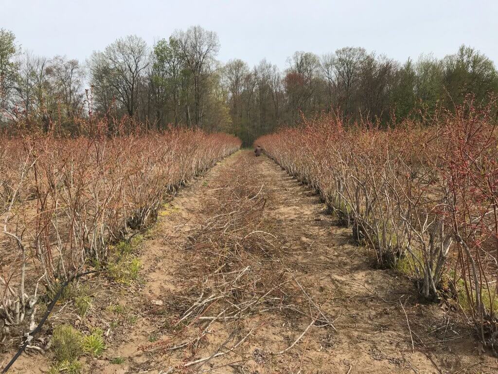
    Heavy pruning in 2016.
    Most years, bushes were pruned ~30% to maintain an ideal size and shape.
    Pickers were educated in how to pick cleanly and dropped / culled fruit was collected and buried.

    2. Selecting a sprayer suited to blueberries

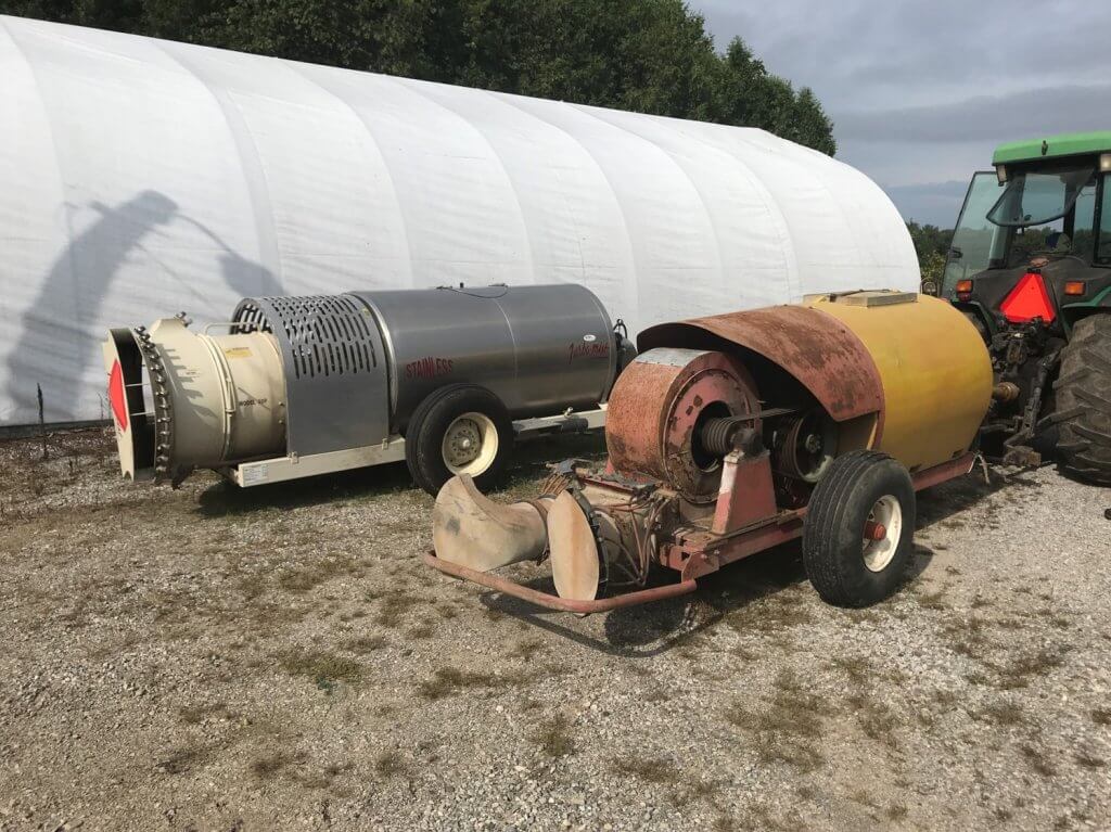
    In 2018, the operation replaced its aging KWH air-shear sprayer with a low-profile axial-fan sprayer equipped with conventional hydraulic nozzles.

    The KWH sprayer had been designed for standard fruit-tree canopies. It generated air speeds greater than 100 mph and produced an Extremely Fine spray quality. These characteristics were poorly matched to the shorter, denser architecture of highbush blueberries.

    The growers considered a cannon-style sprayer that could treat several rows in one pass. However, their priorities were improved coverage and reduced off-target loss. They therefore selected a low-profile sprayer and continued to travel every row.

    The new sprayer provided several immediate benefits:

    • Better control over droplet size and liquid distribution
    • Air direction and volume better suited to the canopy
    • Greater reliability
    • Lower fuel use
    • Less noise
    • Elimination of leaks
    • Positive nozzle shutoff at row ends
    Fore: An old KWH air shear sprayer. Rear: Low profile axial sprayer with conventional hydraulic nozzles.

    Correcting leaks and eliminating continued discharge during turns reduced spray use by approximately 20% before any further rate adjustment was made.

    3. Matching the application to the canopy

    Crop-Adapted Spraying, or CAS, provides a structured way to adjust an airblast application to the size, density, and shape of a three-dimensional crop canopy.

    Several established dose-expression systems perform a similar function, including Tree-Row Volume, PACE+, and DOSAVIÑA. Although each has value, adoption can be limited by crop-specific requirements or complicated calculations.

    CAS formalizes adjustments that experienced applicators often make informally, such as:

    • Turning individual nozzles on or off according to canopy height
    • Redistributing flow among nozzle positions
    • Adjusting travel speed for canopy density
    • Changing air output and direction to improve penetration and reduce loss

    The blueberry sprayer was calibrated by adjusting air energy and direction, travel speed, nozzle selection, and liquid distribution. Water-sensitive paper was placed throughout the canopy to confirm that the revised settings provided acceptable coverage.

    The working coverage targets were:

    • At least 85 deposits/cm²
    • Approximately 10% to 15% surface coverage
    • Achievement of these targets in at least 80% of the sampled canopy
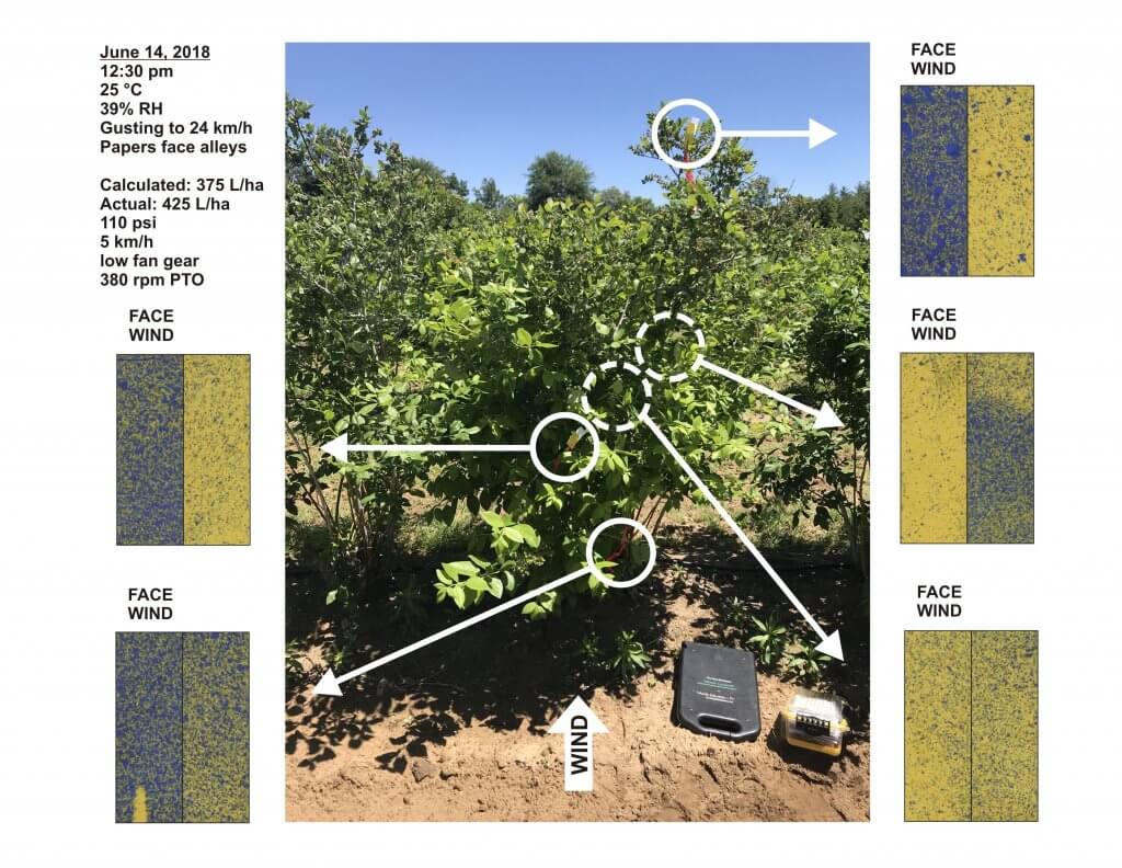
    Example of water sensitive paper coverage on a windy day (worst case scenario) in June, 2018.

    During the first season, coverage was reassessed every few weeks from April through June as the canopy developed.

    Spray volume / Pesticide

    Once the new sprayer was calibrated to the managed canopy, spray volume declined from approximately 1,000 to 400 L/ha. The concentration of formulated product in the spray mixture remained unchanged. Instead, the calibrated sprayer allowed each tank to treat a larger area while maintaining the required canopy coverage.

    Before the sprayer replacement and adoption of CAS, the operation applied approximately 78,260 L of spray mixture annually. Average annual water savings were approximately 55,173 L, equivalent to a 70.5% reduction. That’s almost 1/2 a million liters in 10 years.

    The lower spray volume also saved an estimated 15 hours of filling and spraying each year. This reduced labour and equipment time while potentially reducing operator fatigue and exposure associated with mixing and loading

    Pesticide costs were compared annually with the farm’s 2017 program using updated product prices. On that basis, the average savings were approximately:

    • $5,850 CAD per year
    • 63% of the equivalent pesticide cost

    Pest and Disease Monitoring

    The growers retained responsibility for product selection and application timing. Products were rotated, and treatment decisions were made according to integrated pest management principles.

    Air-induction hollow-cone nozzles were installed in the uppermost nozzle positions. The larger droplets produced at the top of the spray plume were more likely to settle if they passed over the canopy, reducing the potential for off-target movement

    SWD monitoring

    Spotted-wing drosophila traps were monitored weekly from 2018 through 2020. Three traps were placed within the blueberry crop and one was placed in an unmanaged wild host along an adjacent treeline.
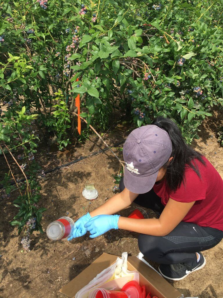
    Regional monitoring provided comparisons with other horticultural operations:

    • Up to 16 berry and tender fruit sites in 2018
    • Approximately 10 to 12 sites in 2019
    • Four blueberry, raspberry, and cherry sites in 2020

    Average SWD captures were higher at surrounding conventionally managed sites in 2018 and 2020. Captures were higher in the CAS planting in 2019. Across the three monitoring years, the overall difference was negligible.

    Trap capture does not necessarily predict the amount of fruit damage. The growers therefore also tested harvested berries regularly. SWD damage remained within commercially acceptable limits, and the growers reported satisfactory disease control.

    Because the monitoring was not replicated or subjected to statistical analysis, it cannot establish that CAS provided equivalent control under all conditions. It does indicate that, on this farm, lower spray volumes and pesticide use were compatible with acceptable commercial control.

    Yield and seasonal conditions

    Yield varied for reasons unrelated to sprayer calibration, including pruning intensity, labour availability, harvest timing, market conditions, and weather.

    • 2016: The baseline before any management changes. The farm harvested 12,076 flats, each containing approximately 9 lb of fruit.
    • 2017: Following the initial canopy-management changes, harvest increased to 18,335 flats; an increase of approximately 50%.
    • 2018: Yield remained essentially unchanged in the first year of CAS.
    • 2019: Harvest began about one month late. Low blueberry prices also prompted the farm to stop harvesting approximately one month early. Allowing for the shortened harvest period, production appeared comparable with previous years.
    • 2020: Anticipated shortages of seasonal labour during the COVID-19 pandemic led the growers to prune heavily and deliberately reduce the crop.
    • 2021: Little pruning was needed following the previous year’s heavy pruning. The resulting denser canopy, combined with unusually high precipitation, contributed to serious anthracnose pressure. More fungicide applications were made than in any other study year, although CAS-calibrated rates and settings were maintained.
    • 2022 and 2023: Spotted-wing drosophila pressure was low, anthracnose pressure was moderate, and production conditions were relatively typical.
    • 2024: Heavy rainfall contributed to an early start and finish to the season, but yield remained near normal.
    • 2025 and 2026: The seasons were generally typical, with no major production disruptions.

    These annual differences demonstrate why pesticide use, pest pressure, yield, and weather should be interpreted together. A low-use year may reflect either improved application efficiency or low pest pressure. Likewise, a high-use year may reflect exceptional disease pressure rather than a failure of the calibration method.

    Additional benefits reported by Falcon Blueberries

    The operation identified several benefits beyond direct pesticide and water savings:

    • Reduced pesticide use provided a positive response to questions from U-pick customers.
    • Lower environmental pesticide loading aligned with the growers’ production philosophy.
    • During a regional fungicide shortage in 2018, the farm had enough unused product to return some to the distributor.
    • Reduced early-season disease damage decreased the amount of fruit removed on the packing line.
    • Fewer tank fills reduced labour, machinery time, and interruptions during spraying.

    Practical implications for all highbush blueberry growers

    The results from this farm should not be interpreted as a recommendation to reduce pesticide rates by a fixed percentage. The important principle is to match the application to the canopy and confirm performance. Growers considering a similar approach should:

    1. Manage the canopy. Maintain a reasonably open and consistent target through regular pruning.
    2. Correct obvious sources of waste. Repair leaks, confirm positive nozzle shutoff, and prevent discharge during turns.
    3. Match the sprayer to the crop. Adjust fan output, air direction, nozzle positions, droplet size, travel speed, and liquid distribution.
    4. Measure coverage. Use water-sensitive paper or another suitable method at representative locations and depths.
    5. Reassess as the canopy changes. Settings that work before bloom may not be appropriate after the canopy fills.
    6. Respect the label. Do not reduce application volume or pesticide use below label requirements.
    7. Document the results. Record settings, weather, water volume, products, pest pressure, coverage, and crop response.
    8. Make changes incrementally. Confirm coverage and control before adopting larger reductions.

    The achievable reduction will vary with canopy size and density, sprayer design, product requirements, pest pressure, weather, and the applicator’s ability to verify coverage.

    Conclusion

    Over ten years, this southern Ontario blueberry operation substantially reduced spray volume and pesticide costs while maintaining commercially acceptable pest and disease control. These outcomes resulted from a coordinated production-system change rather than from a single calibration adjustment. Canopy management created a more accessible target, the new sprayer provided better control of air and liquid, and Crop-Adapted Spraying supplied a repeatable method for confirming coverage.

    The case study demonstrates that meaningful pesticide savings are possible when rate adjustment is based on crop structure, appropriate application technology, and measured coverage. It also reinforces an important limitation: results from one farm should guide further evaluation, not replace on-farm calibration, label compliance, or local validation.

    Here’s a narrated PowerPoint presentation of this study (includes data up to 2020):

    The monitoring portion of this project was funded by Niagara Peninsula Fruit and Vegetable Growers Association, Ontario Grape and Wine Research and Ontario Tender Fruit Growers in collaboration with private consultants.

  • Spray Window – Can you plan a spray week?

    Spray Window – Can you plan a spray week?

    Plan the day. Weigh the risks. Finish the job.

    Spray Window is a strategy game about spray planning. You have one sprayer and six working days of changeable weather. Depending on your role, you manage your own fields or a list of clients’ jobs.

    Each turn is one day. Read the forecast and what each field needs, choose which jobs to do and in what order, set up the sprayer, and see how the day unfolds. There’s no single right answer.

    It’s what every operator learns on the job: assess the work, plan ahead, weigh risk against reward, and get as much done as you safely can. A week takes about 20 minutes and plays best on a tablet or computer. At the end, a debrief shows what your decisions cost, what they saved, and how a benchmark operator planned the same week.

    Why a game?

    Sprayer training usually covers drift, Delta T, inversions, spray quality, water volume, travel speed one at a time. On a real morning they all arrive together, along with crop stage, a closing window, a neighbour, and someone waiting on the work.

    Those decisions rarely have one correct answer, so they’re hard to teach in an article or test with a quiz. An owner facing a closing disease window might reasonably accept more drift risk than a custom applicator whose business depends on reputation. Both may be making a sound call.

    A simulation lets you decide, live with the consequences and try again. In Spray Window, the opponent is the weather and the clock, not another player. And, of course, it’s a fun 16-bit style that reminds me of a lot of wasted quarters in my youth.

    How it plays

    The game is set in Ontario mostly on corn, soybeans and winter wheat, with canola, white beans, sugar beets, processing tomatoes and potatoes in some weeks. Every week is a new combination of fields, crops, pests and weather, in one of three seasons.

    Choose your role (owner-operator or custom applicator) and your level, outfit your sprayer on a limited budget, pick your tires, and dive in. The weather changes, and there are surprises to deal with.

    There are three levels.

    • Beginner is a quiet week of seven fields: honest work orders, no surprises, no tank cleanouts and nobody pushing you to spray, and the sprayer comes ready to go.
    • Intermediate has ten fields and adds wind gusts, an interruption, wet ground, cleanouts and people leaning on you.
    • Expert is the full game. Your week is saved each morning, so you can stop and come back to it.

    Micron Woman is back to be your guide.

    Choose your role and level – the scenarios change accordingly.

    Spring

    In mid-May, jobs include herbicide and fungicide in wheat, a pre-emergence herbicide before the corn comes up, a burndown ahead of soybean planting, and insecticide for cereal leaf beetle and black cutworm at threshold.

    Early Summer

    In mid-June, jobs include fusarium head blight at wheat flowering, a Group 4 herbicide before the corn’s crop-stage limit, post-emergence herbicides in soybeans, and armyworm in wheat.

    Mid-Summer

    In late July, jobs include tar spot at corn tassel, white mould and soybean aphid in soybeans, western bean cutworm, and a pre-harvest herbicide as wheat dries down. 

    Drift

    Every field borders something sensitive: open water, a neighbour’s home and garden, beehives in a flowering hedgerow, a vineyard or a certified organic farm. Each responds as it would in real life.

    When water or habitat is downwind, the label may require an unsprayed buffer, and coarser sprays shrink it. Coarser sprays also cut drift sharply, because each step coarser roughly halves the fine droplets that drift, but fungicides and insecticides lose some coverage, so more water helps them. Heat brings another risk: after application, dicamba can turn to vapour and move off target whatever the nozzle. In June, a cooler day or a pass after the heat of the day may be the safer call.

    Sometimes, not spraying is the right move.

    Outfit your sprayer for the week ahead.

    High scores, weekly scenarios and feedback

    Money keeps score. Beside your money, a second readout shows whether you’re ahead (▲) or behind (▼) the benchmark operator playing the same week. Every off-label pass is a label strike and a fine, so bad calls sting right away. If your balance falls below zero, you’re broke and the week ends with zero points.

    A score of 1,000 means you finished as well off as the benchmark. Both roles use the same yardstick, and weeks are drawn from scenarios of similar difficulty, so scores are comparable. Each level has its own benchmark and its own high scores, so beginners compete with beginners.

    Ranks are awarded as follows: 

    • Apprentice (0-499)
    • Operator (500+)
    • Pro (800+)
    • Ace (950+)
    • Legend (1,100+)
    Get your rank and scorecard. See what you might have done differently.

    At the end of the week you get your report card. “Turning points” shows the three decisions that cost you most and what the forecast would have allowed instead. If you want to understand how the game balances all these variables, check out the (assumptions) button.

    Enter your initials arcade-style. Your score is sent to the leaderboard automatically and once we review it, the leaderboard updates. Playing a downloaded copy? Email the code from the end screen to jason@sprayers101.com. Something odd, or a call you’d question? Copy the code and send it with a note: your exact week can be replayed. Only a week’s first play counts; “Play this week again” is for practice.

    Thanks to Dr. Ian McDonald for the inspiration to build a game. Ready to play?

    High Scores

    1. 1RKLegendCustom applicator1,102points
    2. 2JAYAceOwner-operator1,072points
    3. 3RKAceCustom applicator994points

    See the full leaderboard

    Version Updates:

    Updated November 6, 2026: Three levels, Beginner, Intermediate and Expert, each with its own high scores. A week in progress is saved on your device, so you can finish it later. And on still mornings, listen for a train in the distance. Scores from earlier versions count as Expert.

    Updated November 5, 2026: Refills and water volume now add up correctly, so more water never makes a job finish sooner (thanks, Lucas). Each job card now shows how the product moves, its Group and its rainfast time, and the day plan warns when rain could wash it off. Micron Woman’s tutorial is clearer and shorter. Scores from earlier versions still count.

    Updated November 2, 2026: Spray quality and walking the edges rebalanced so careful decisions pay off more, and the top three scores now appear on the title screen between rounds. Scores from earlier versions still count.

  • How Much Pesticide in the Tank?

    How Much Pesticide in the Tank?

    Sprayer math can be intimidating, but the effort gives solid value. When combined with a calibrated sprayer you reap the following benefits:

    • Determine how much spray mix is required to apply the intended rate.
    • Estimate how much crop protection product must be ordered for the season.
    • Populate spray records which allow you to review practices, respond to enquiries and satisfy traceability requirements.

    There are many ways to perform sprayer math, and you need only look to local pesticide safety courses, industrial catalogues, and extension resource centres for examples. If you’re already comfortable with your current method, don’t mix and match with others. Sprayer math is a series of related calculations that employ constants to keep the units straight. It’s all or none.

    Walkthrough

    Let’s start with the classic, US Imperial formula for calculating the sprayer output. We’ll weave in Metric, later. This base formula can be adjusted to allow you to solve for any factor, as long as you’re only missing one piece of information. Turns out your high school teacher was right – you DO need algebra.

    GPM = [GPA x MPH x W] ÷ 5,940

    In this case, you can determine an output rate (GPM – gallons per minute). You’ll need to know your target volume (GPA – gallons per acre), your average travel speed (MPH – miles per hour) and your nozzle spacing (W – which is width in inches). The number “5,940” is a constant that handles all the unit conversions. If you divide the GPM by the number of nozzles on your sprayer (assuming they are all the same rate), you can hone in on the ideal nozzle size.

    But, as we noted earlier, you can do a lot more with sprayer math than just pick the ideal nozzle size. The rest of this article includes examples of both Metric and US Imperial formulae, but watch out for unit conversions. If at any time you don’t see the units you’re looking for, you can consult our unit conversion tool.

    Grab your calculator – it’s math time!

    Don’t be intimidated. With a little practice, sprayer math gets easier and it’s always worthwhile. The real trick is navigating unit conversions.

    Step 1 – How large is the area you need to spray?

    Multiply the length of the area you plan to spray times the width. If you are using metres, then divide the product by 10,000, which is the number of m2 in a hectare (ha). For feet and acres, divide by 43,560 which is the number of ft2 in an acre (ac):

    Step 2 – How much product is needed to spray the area?

    Consult the rate(s) shown on the label. In Canada, rates are often based on planted area (E.g. hectares). In Australia and New Zealand, they may be based on row length (not covered in this article). If you measure your area in acres, you’ll have to convert the rate by multiplying by a constant: 0.4.

    product-per-area

    Now multiply the area you want to spray (step 1) by the rate (step 2).

    product-per-area2

    Step 3 – How far can you go on a full tank?

    You know your sprayer output (determined through calibration) so you divide that into your tank size. Watch your units:

    full-tank-distance

    Step 4 – How much pesticide per tank? 

    Multiply the area that can be sprayed per tank (Step 3) by the pesticide rate (Step 2). Again, watch your units:

    pesticide-per-tank

    Step 5 – How much area is left to spray?

    Just subtract what you’ve already sprayed from the total area.

    area-left-to-spray

    Step 6 – How much pesticide in the last, partially-full tank?

    Multiply the area you have left to spray (Step 5) by the pesticide rate (Step 2). Yes, watch your units:

    pesticide-partially-full-tank

    Step 7 – How much spray mix will I need for the partial tank to finish spraying the total area?

    Multiply the area you have left to spray (Step 5) by the sprayer output (determined through calibration). Guess what? Watch your units:

    spray-mix-for-total-area

    Sample problems

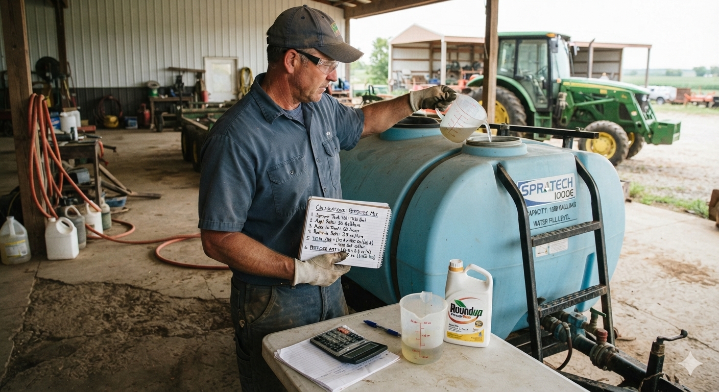
    Time to test your knowledge. Let’s suppose you want to apply a product rate of 3 L/ha to your blueberries. You calibrate your sprayer and determine your output to be 50 L/ha. Your tank holds 400 L of spray mix. Your planting is 500 m long and 200 m wide.

    Q1 – How large is the area you need to spray?

    area-to-spray

    Q2 – How much product is needed to spray the area?

    product-to-spray-the-area

    Q3- How much area can be sprayed on one tank?

    area-on-full-tank

    Q4 – How much product should be added to a full tank?

    product-needed-full-tank

    Q5 – After the tank is empty, how much area is left to spray?

    area-left

    Q6 – How much product to add to the last, partially full tank?

    product-partially-full-tank

    Q7 – How much spray mix will be needed to finish spraying?

    spray-mix-to-finish-spraying

    Tank mix calculator

    You might feel we buried the lead by adding this calculator to the end of the article. It’s important for a sprayer operator to understand the math required to interpret labels and calculate tank mixes, so hopefully you read and understood the process before you got here. And now that you have, this is a very helpful tool. Try it online, or download a standalone version.

    Notable exceptions

    Certain situations aren’t covered in this article. If you are spraying a greenhouse, the math is different. If you are performing a banded application, the math is different. And, if you’re an airblast operator trying to reconcile why a pesticide label uses planted area rather than canopy volume for its rates, you’re in for some additional reading.

  • Determining Airblast Travel Speed – The “Air Displacements” Method

    Determining Airblast Travel Speed – The “Air Displacements” Method

    What is the “right” speed to drive when spraying?

    Airblast sprayer operators must know their average travel speed to calculate how much pesticide and time is required to complete a spray job. Note that it’s an average, not a constant, because travel speed is significantly affected by ground surface conditions (e.g. slippage), grade (e.g. hills) and the weight of the rig (e.g. as spray mix is depleted).

    The pursuit of productivity and the unchallenged status quo of traditional spray volumes, blinds many operators to the fact that travel speed is a critical factor in focusing air energy on the target canopy. As long as droplets are small enough to be entrained and directed by the air, we believe that optimizing the fit between air energy and the target canopy leads to the most frugal and effective use of spray mix and should therefore dictate travel speed. If that speed proves to be painfully slow, or terrifyingly fast, then a mismatch is revealed between the sprayer design and the operational conditions and the overall spraying strategy should be reconsidered.

    This article describes a method for modelling an ideal travel speed. It can be used as a sanity check for existing operations or for those seeking to evaluate the fit of a new airblast sprayer. However, this method can only approximate travel speed. A true optimization of sprayer settings will require fine tuning using the ribbon method and, ultimately, coverage feedback from water sensitive paper (see here and an older article here). We’ll begin with how to measure average travel speed.

    How to measure average travel speed

    Beware the tractor speedometer or rate controller that monitors wheel rotations; both can be fooled by changes in wheel size, tire wear or slippage. GPS or radar-based speed sensors are the most accurate method.

    Those that prefer a manual method can follow this classic protocol for determining average travel speed:

    1. Go to a row that is representative of the terrain in your planting. Measure out a distance of 50 m (150 ft) and mark the start and finish positions with wire marker flags.
    2. Fill the sprayer tank half full of water.
    3. Select the gear and engine speed in which you intend to spray. If using a pull-behind sprayer, ensure the PTO is running or you could introduce errors.
    4. Bring the sprayer up to speed for a running start and begin timing as the front wheel passes the first flag. This is far easier when there are two people.
    5. Stop the timer as the front wheel passes the second flag.
    6. Stay out of any ruts and run the course two more times.
    7. Determine the average drive time for the three runs (i.e. the sum of all three times in seconds divided by three).
    8. Finally, calculate travel speed using one of the following formulae, depending on preferred units:

    Ground Speed (km/h) = Average drive time for 50 m (s) ÷ 13.9 (a constant)

    Those that prefer a less accurate but convenient hack can download any smartphone speedometer app that can calculate an average (similar to a runner’s GPS wristwatch). Fill the sprayer tank half full and drive a representative section of your operation with the fan on and the spray off. Consult the phone for your average speed for each pass. Take a screen shot and email it to yourself as a time-stamped component of your spray records.

    The “Air Displacements” method

    Dwell time

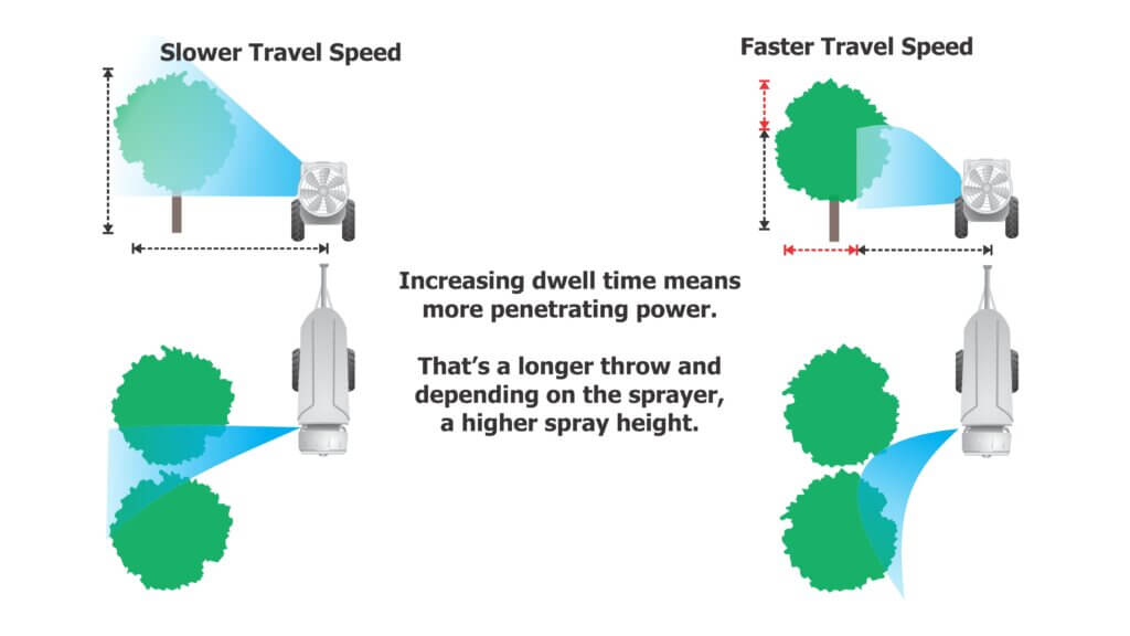
    Airblast sprayers use fans to move a volume of air at a certain speed, often measured in m3/hr or ft3/min. Imagine that volume of air as a three dimensional shape extending from the air outlet over a distance. Likewise, imagine the void between the sprayer outlet and the target canopy as a three dimensional shape penetrating roughly halfway into that canopy (assuming we intend to spray every row).

    How long must the sprayer dwell in one spot before it pushes all the intervening air out of the way and replaces it with spray-laden air? If the sprayer drives too slowly, it will wastefully push spray through and beyond the target (i.e. blow-through). If the sprayer moves too quickly, the spray will not have an opportunity to penetrate the target canopy and most certainly not reach the highest point. This concept of focusing air energy using travel speed is called Dwell Time.

    We want to calculate the volume of air the sprayer generates, compare that to the volume we want displaced, and then determine how fast we must drive to optimize the fit. We can do all this with a tape measure, an anemometer, and a partner to record the data and do a little math.

    1. Measure air outlet area

    With the sprayer safely off, measure the area of the air outlet(s) on one side of the sprayer. We’ll use a Turbomist 30P Low Drift Tower (below) as an example. There are two air outlets that are 5 cm wide by 150 cm high for a total area of 0.075 m2 on each side. Be sure to look inside the outlet for any irregularities like baffles or obstructions intended to block air. Subtract those areas from the total. Don’t worry about small things like nozzle bodies.

    For rectilinear outlets: Height (m) x width (m) = Area (m2)

    For circular outlets: 3.14 x radius2 (m) = Area (m2)

    The air outlet on this Turbomist 30P Low Drift tower sprayer is 5 cm wide by 150 cm tall for a total area of 0.075 m2.

    2. Measure air speed

    First, a few safety warnings: High speed air is loud and can carry debris, so always wear ear and eye protection and respect the hazards inherent to working with air-assist sprayers. Only use an anemometer rated for at least 160 km/h (100 mph) (e.g. here). Do not use a handheld weather meter such as a Kestrel because the impellor could be destroyed and become dangerous shrapnel.

    Use an anemometer rated for at least 160 km/h (100 mph) (e.g. here). Do not use a handheld weather meter such as a Kestrel because the impellor could be destroyed and become dangerous shrapnel.

    Bring the fan up to speed and holding the meter about 25 cm (10 in.) from the outlet, measure the air speed at several locations along the air outlet both vertically and horizontally. We calculate an average speed because many air outlets do not produce uniform air speed or volume along their outlets. For this example, we measured four locations along the air outlet on both sides of the sprayer and saw significant differences. We did this both in low and high gear (see table below).

    High GearHigh GearLow GearLow Gear
    Location Along OutletLeft Side (m/s)Right Side (m/s)Left Side (m/s)Right Side (m/s)
    Top 1/441.180.342.924.6
    Upper34.932.226.430.8
    Lower30.830.024.026.4
    Bottom 1/433.540.226.831.3
    Average35.145.730.028.3
    Anemometer readings from the low drift tower sprayer outlets, on left and right side, in high and low fan gear. Four readings from bottom to top to determine the average. Readings taken 25 cm from edge of outlet and PTO set to 540 rpm.

    Multiple air outlets

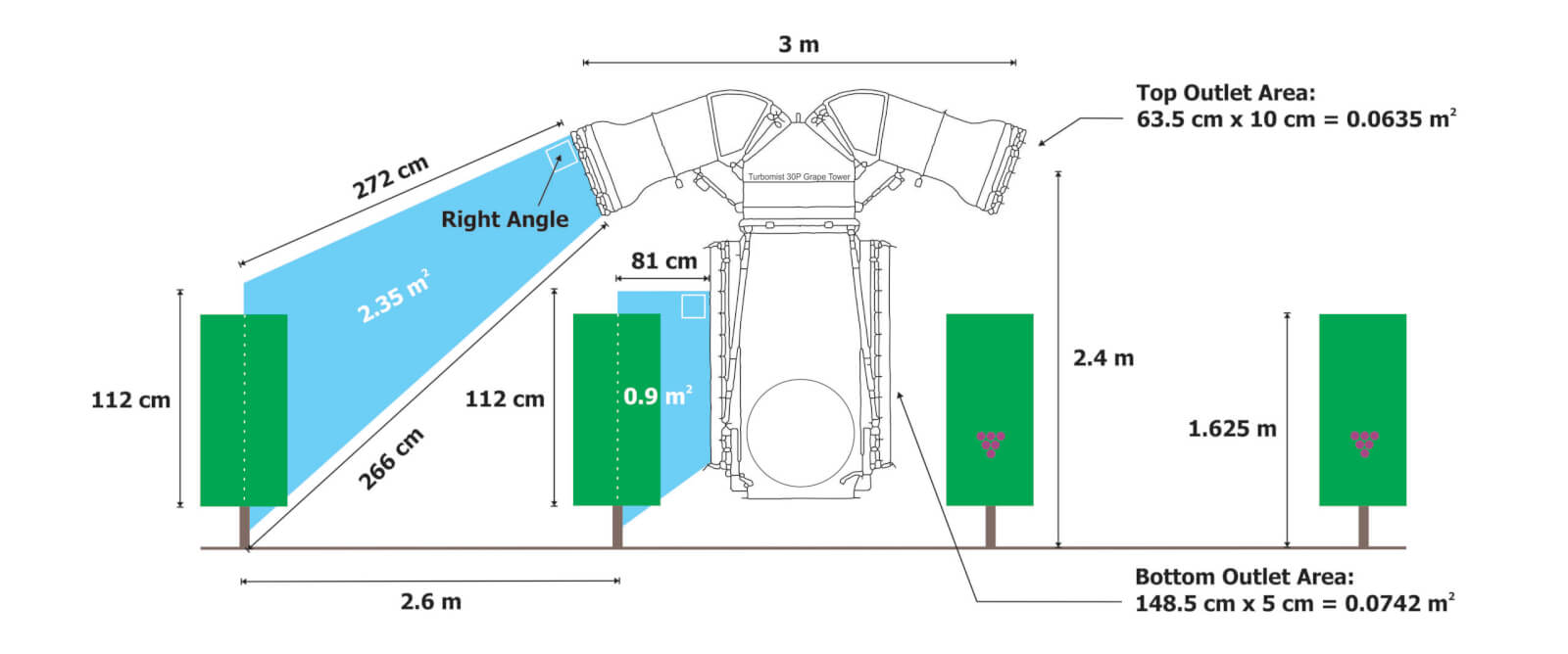
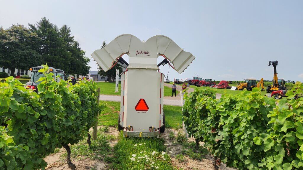
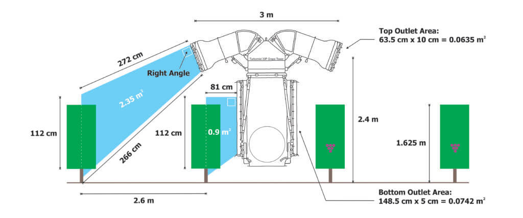
    Before we continue with the method, let’s change sprayers to this Turbomist 30P Grape Tower (below). The design is intended to spray adjacent rows from the vertical outlets (5 cm x 150 cm = 0.075 m2) along the tower. The upper, inverted outlets (10 cm x 63.5 cm = 0.0635m2) throw spray over the adjacent rows and cover the outside rows. The intention is to improve productivity by covering four rows of grape (or possibly three) per pass.

    The Turbomist 30P Grape Tower Sprayer is a multirow system intended to drive every third or fourth row.
    Lower, vertical ducts are 5 cm x 150 cm = 0.075 m2
    Upper, inverted ducts are 10 cm x 63.5 cm = 0.0635m2

    However, when we consider this design through the Air Displacement lens, it’s almost like having two sprayers performing two jobs simultaneously. The vertical outlets and the upper, inverted outlets are different shapes. Further, their position (distance and angle, as the top outlets are angled back more aggressively) relative to their respective target canopies are significantly different. How fast must this sprayer drive to optimize the fit? Do we have to compromise coverage and incur drift and waste from one set of outlets to accommodate the other set? The manufacturer has worked to address this potential issue by partitioning the majority of the air energy to the top outlets, but let’s see how that affects travel speed.

    3. Total volumetric flow

    Having already measured the outlet area, we then measured average air speed (see table below).

    High GearHigh GearLow GearLow Gear
    Location Along OutletLeft Side (m/s)Right Side (m/s)Left Side (m/s)Right Side (m/s)
    Top Outlet27.026.527.026.0
    Bottom Outlet12.013.010.512.5
    Average anemometer readings (n=4) for top and bottom outlets, on left and right side, in high and low fan gear. Readings taken 25 cm from edge of outlet and PTO set to 540 rpm.

    Now we can use these two values to determine how much air the sprayer generates by calculating total volumetric flow. We first have to convert air speed from m/s to m/h to make the units work, so just multiply it by 3,600. Then we multiply that by the outlet area and we get the table below.

    Average air speed (m/s) x 3,600 (a constant) = Average air speed (m/h)

    Average air speed (m/h) x Outlet area (m2) = Total volumetric flow (m3/h)

    High GearHigh GearLow GearLow Gear
    Location Along OutletLeft Side (m3/h)Right Side (m3/h)Left Side (m3/h)Right Side (m3/h)
    Top Outlet6,172.06,058.06,172.05,944.0
    Bottom Outlet3,240.03,510.02,835.03,375.0
    Total volumetric flow for top and bottom outlets, on left and right side, in high and low fan gear, with PTO at 540 rpm.

    4. Target volume to displace

    Now that we know the volume of air the sprayer generates, let’s determine the volume of air we need to replace with that spray laden air. This is really the only tricky bit because you have to picture a cross section and then measure the shape. See the illustration below.

    For the bottom outlet, it’s simple. The outlet is 81 cm from the grape panel and the grape panel is 112 cm high. We calculate the area of a rectangle by multiplying length by width, so:

    Length (cm) x Width (cm) = Area (cm2)

    However, the sprayer design makes the top outlet’s job trickier to figure out. This isn’t a rectangle, it’s a “quadrilateral”. We get this odd shape when either the sprayer outlet or the target canopy are significantly taller than the other. Fortunately this one has a right angle so we don’t have to brush off our high school trigonometry textbooks. Instead, we can lean on the internet using this link and plug in the values. As we can see below, the cross sectional areas spanning from the outlets and the middle of the target canopies are 0.9 m2 for the bottom outlet, and 2.35 m2 for the upper outlets.

    This gives us a cross sectional area, but we need to convert that to a volume so we can compare the air generated to the air needed. To do that, we multiply the cross sectional area by 100 m, representing how much air would be needed over 100 m of row length. The formula and the results are presented below.

    Cross sectional area (m2) x 100 m of row length = Target displacement volume (m3)

    OutletTarget Displacement Volume (m3)
    Top Outlet235.0
    Bottom Outlet90.0
    Target displacement volume for each outlet over 100 m of canopy row.

    5. Displacement rate

    We see the target displacement volumes for each outlet are significantly different. Assuming the air from the upper outlet maintains its integrity and reaches its target canopy without being blown off course, it must produce enough air energy to fill more than twice the displacement volume of the lower outlet. We can see from the earlier calculations that it does produce almost twice the total volumetric flow. But is it enough? To know we must calculate the Displacement Rate for each outlet. Let’s just focus on the left side of the sprayer in high gear.

    Total volumetric flow (m3/h) ÷ Target Volume (m3) = Displacement Rate ( displacements/h)

    OutletDisplacement Rate (displacements/h) for left side of sprayer in high gear
    Top Outlet26.25
    Bottom Outlet36.0
    Displacement rates for the outlets on the left side of the sprayer in high gear.

    So we see that the outlets at the top of the sprayer, if stationary, could displace the target volume of air 26.25 times an hour. However, the lower outlet would displace its target volume 36 times in that same hour. We see that we might have a problem. But this is for a stationary sprayer and not a sprayer in motion. The last step gives us what we came here for.

    6. Ideal travel speed

    We can now determine the ideal travel speed for this sprayer using that same 100 m row length.

    [Displacement rate (displacements/h) x 100 m of row length] ÷ 1,000 (a constant) = Ideal travel speed (km/h)

    OutletIdeal travel speed (km/h) based on left side of sprayer
    Top Outlet2.6
    Bottom Outlet3.6
    Ideal travel speed for each outlet on the left side of the sprayer in high gear.

    As we stated at the beginning of this article, this is only a model. It doesn’t account for canopy density and assumes the spray laden volume of air produced by the sprayer can reach the target intact over a given distance. However it does indicate that there is a potential issue that will lead to either over spraying the adjacent row (slower travel speed) or under spraying the distant rows (faster travel speed) which could lead to waste, drift and poor coverage.

    In the image below, we chose to drive close to 2.6 km/h in high gear. No effort was made to adjust the liquid flow (i.e. change the nozzles) so there was too much spray volume here, but we can see the losses on the left (upwind) side, and the blow-through three rows over on the right (downwind) side. Leaving aside the excessive liquid volume, we could drive faster or reduce the fan gear to reduce the blow-through on the adjacent rows, but we may go too fast (or reduce the rate of air displacement) for the upper outlets to reach the target. We can already see the integrity of the upper-left outlet breaking down as it sprays into the wind.

    Testing a travel speed. No effort was made to adjust liquid flow, which is excessive here. Cross wind was from the left to the right in the image. Photo by Corey Parker (Instagram: _parkerproductions)

    Take home

    An ideal travel speed for an airblast sprayer is more than just being productive. The spray must reach and penetrate the target. If this requires dangerously high speeds, or if you simply can’t move slowly enough, it suggests a problem with the spraying strategy. Changes will have to be made to the sprayer, the target canopy, or even the weather conditions you’re willing to spray in. Getting the job done quickly should not compromise the quality of the job. Use this method to re-evaluate your practices, or to assess the capabilities of candidate sprayers if you’re considering a new purchase. Be sure to confirm what this model is telling you using some coverage indicator, such as water sensitive paper.

    Calculator

    Now that you’ve read through the process, you can try this online calculator designed to make the process a little easier. The embedded illustrations are there for general guidance, and may not reflect the sprayer design, but the calculations work. Recognize that while this calculator will provide an idealized travel speed based on the data entered, it cannot judge whether the outcome is realistic. Obviously a recommendation to drive 25 km/h is unrealistic, but it does alert the user to the fact that the sprayer is overpowered. Try it out!

    Dr. David Manktelow, Applied Research and Technologies Ltd., is gratefully acknowledged for patiently explaining the concept of “Air Displacements” to the author.

  • Greenhouse Foggers

    Greenhouse Foggers

    Greenhouse application equipment spans from the humble squirt bottle, to gas-powered foggers, to robots equipped with hydraulic vertical booms. The variety of spray equipment available reflects a variety of needs, just as a carpenter’s toolbox contains different tools designed to do different things. In order to get the most out of foggers and misters, it’s important to understand how they differ from “conventional” hydraulic spraying.

    A greenhouse robotic vertical boom sprayer.
    A greenhouse robotic vertical boom or “tree” sprayer

    Mechanical and Chemical Spread

    For many greenhouses, water is the carrier that dilutes and delivers the chemistry to the target. Water has a high surface tension and tends to bead on target surfaces. Dr. Heping Zhu (USDA, Ohio) created some amazing videos using controlled water droplets and both waxy and hairy leaves. In first video we see how water beads up on a waxy leaf, and as it evaporates, the area touching the leaf surface remains small. In the second, we see the droplet get hung up on a trichome (leaf hair) and evaporate while suspended above the leaf surface.

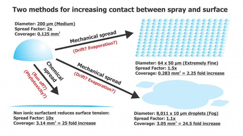
    Neither situation is desirable since the goal of spraying is to maximize the level of contact between droplet and target. Contact can be increased via mechanical spread or chemical spread (see figure below).

    The degree of chemical spread can be increased by adding adjuvants such as non-ionic surfactants to reduce surface tension. In the videos below we see the same controlled droplets with the same volume of liquid, but they now include a non-ionic surfactant. In the first video we see a greater degree of contact with the waxy target surface as the droplet spreads. In the second, the droplet does not get caught by the trichome, but splashes down onto the surface. Some product labels advise the inclusion of adjuvants and others are already formulated with them. In the case of surfactants, be aware of the potential for run-off and phytotoxicity.

    Mechanical spread requires us to break a single, larger droplet into several smaller volumes to increase the degree of contact. This approach usually comes with a caveat about evaporation, but this is rarely a concern in a humid greenhouse. As for the risk of drift, once again, in greenhouses it is a different story than conventional spraying. Spray drift is desirable! Lateral air movement is very important to encourage plant canopy penetration and prevent droplets from merely settling on upward-facing plant surfaces. While some equipment generates its own air, the air currents in the greenhouse are often the primary means for suspended droplets to circulate throughout the space. In either case, air could be considered the carrier instead of water. Too little air flow, or gaps in circulation, will reduce coverage. Too much air flow (specifically, greenhouse air circulation) may cause plants to exhibit stunting.

    Spray Quality (ISO)

    Here’s how ISO/DIS (5681:2019 Equipment for crop protection — Vocabulary 3.2.1) defines the spray quality produced by misters and foggers:

    • (3.2.1.13) MIST: “Spray with volume median diameter between 50 µm and 100 µm.”
    • (3.2.1.14) FOG: “Aerosol spray with volume median diameter under 50 µm where the droplets are effectively suspended in air with little or no settling by gravity.”

    These droplets do not behave like coarser droplets. For more information on droplet movement, survivability, and transfer efficiency, download Purdue Extension’s “Adjuvants and the Power of the Spray Droplet”.

    Water sensitive paper has limited utility when diagnosing coverage from foggers. Sophisticated optical scanners may be able to detect deposits as small as 25 µm, but this is open to debate. Manufacturers do not support the use of papers when quantifying deposits less than 50 µm , and some draw the line at 100 µm.

    In the following image, papers were used to diagnose coverage (from clean water) in a poinsettia greenhouse. The two papers on the right were located in the canopy and sprayed using a thermal pulse fogger and a hardware store style hand pump. The paper on the left was held directly in the path of the fogger while using the smallest nozzle provided with the unit. The spray enveloped the paper (and the person holding it). Close inspection showed tiny deposits, and the SnapCard app detected 4.5% coverage, but this greatly underestimates the actual deposition and does not account for the droplet count.

    UV dyes are the preferred method for analyzing coverage from foggers.

    Fogging and Misting Equipment

    Greenhouse spray equipment can be classified by droplet size, but also by the spray volume they employ.

    High Volume (HV)

    These applications are performed at pressures ranging from 500 to 4,285 kPa (75 to 700 psi) employing flow rates of 3.9 to 5.7 L/min (1 to 1.5 US g/min). They use standard label rates to accomplish a dilute application by broadcasting droplets larger than 100 microns. The goal is to cover all surfaces without incurring run-off. Examples of HV application equipment include backpack sprayers, trailed sprayers and boom sprayers. Practice and self-calibration are necessary to achieve the desired results when using manual HV sprayers.

    Targeted Low Volume (LV)

    These applications are performed at high pressures around 20,685 kPa (3,000 psi) employing flow rates approaching 1 L/min (0.26 US g/min), covering 93 m2 (1,000 ft2). They apply reduced rates over a given area and create droplets between 25 and 100 µm. These are concentrated sprays that do not result in wet foliage. LV applications are particularly good in high-humidity environments, when it is desirable to minimize the moisture on leaves. Examples of LV application equipment include aerosol cans.

    Ultra-Low Volume (ULV)

    These applications employ flow rates approaching 2 L/min (0.52 US g/min), covering 930 m2 (10,000 ft2). They require concentrated solutions, but apply reduced rates per area using droplets less than 25 µm. ULV applications will not raise greenhouse humidity and are a good choice when days are short and nights are long. They are also an excellent way to apply disinfectants for complete space sanitation before starting a new crop. It is important to ensure vents are closed and fans are off during sanitation. Examples of ULV application equipment include total release cans, auto foggers and thermal pulse foggers.

    PulsFOG hand-held ULV cold fogger

    Thermal pulse foggers are unlike other ULV equipment and warrant special consideration. The design of the pulse fogger has remained virtually unchanged since the 1940’s. Smaller, 24 hp machines are used in smaller operations but range up to large 175 hp machines. Tank size ranges from 10 to 50 L, where 10 L should be enough to cover 4,645 m2 (50,000 ft2) in about 10 minutes, depending on crop density. Their range is about 35 m (115 ft) from the point of release.

    Thermal Pulse foggers do not create aerosol using air shear – they use combustion (80 to 100 explosions per second) to shatter spray into a fog and propel it via positive pressure. Heat is a by-product of the engine, making it an unsuitable method for applying biological products.

    However, water-cooled foggers such as Dramm’s Bio Pulse Fogger reduce the exhaust temperature below 100 °C to make the application bio-rational. This has the added advantage of making droplet sizes more consistent and preventing spray from evaporating too quickly before it diffuses to the target.

    Dramm Bio Pulse Fogger.
    Dramm Bio Pulse Fogger

    Using a Fogger

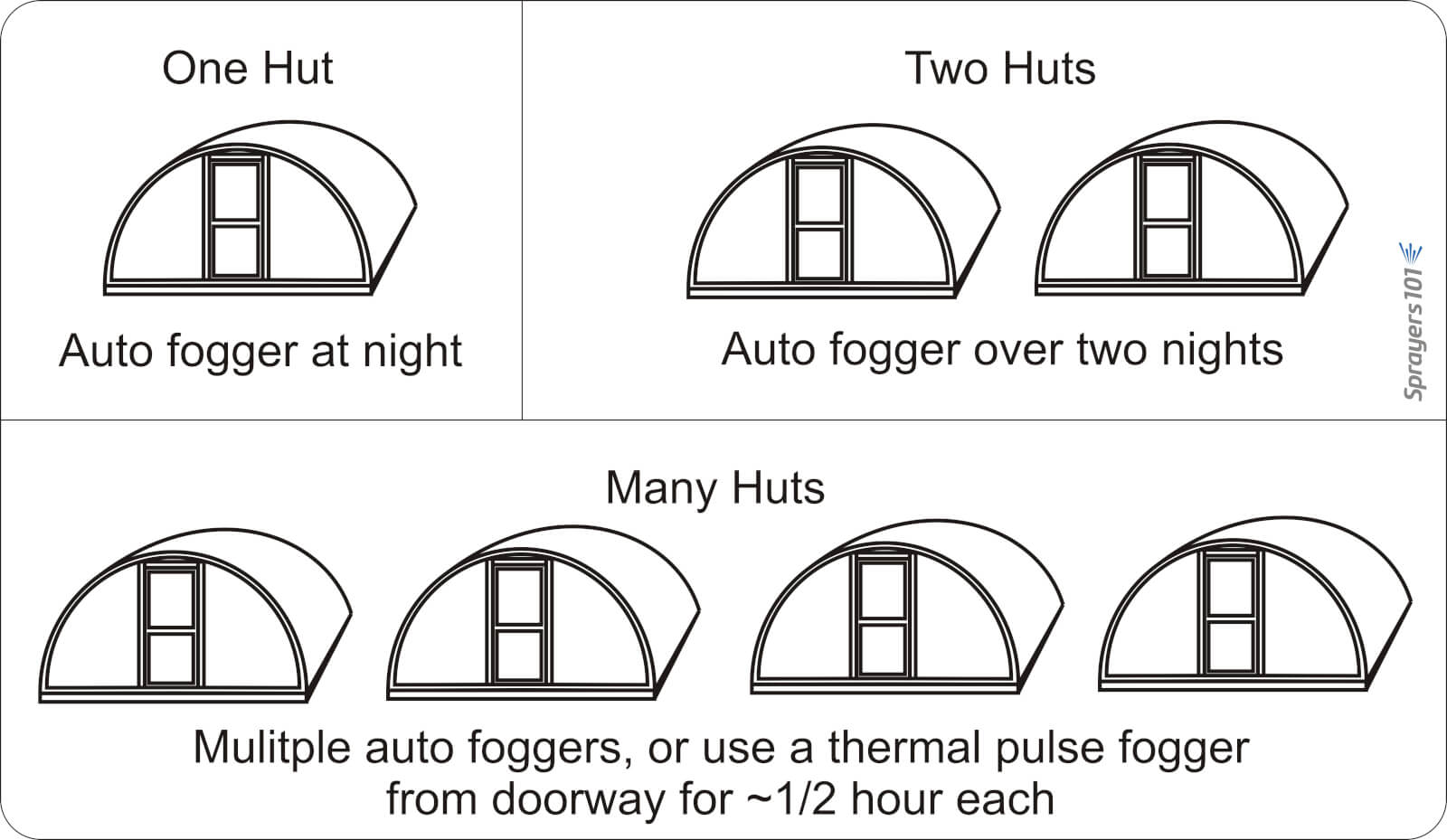
    Dramm recommends that operators use approximately 1 L of carrier in 5 L of spray mix, but a higher proportion of carrier would be required for more viscous products. Start with a full tank of clean, high grade gasoline and once the fogger has been started, run it continuously until the application is complete. Leave it running even when moving between Quonset huts (see below).

    Know when to use a pulse fogger versus an auto fogger. Auto foggers are convenient because the operator can set them and leave. However, in the case of multiple huts, it is more efficient and timely to use a thermal pulse fogger.
    Know when to use a pulse fogger versus an auto fogger. Auto foggers are convenient because the operator can set them and leave. However, in the case of multiple huts, it is more efficient and timely to use a thermal pulse fogger.

    Do not leave the manual fogger running unsupervised as an auto fogger: If they stay stationary, or aim directly at the canopy (as in hydraulic spraying), they could drench and potentially damage nearby plants.
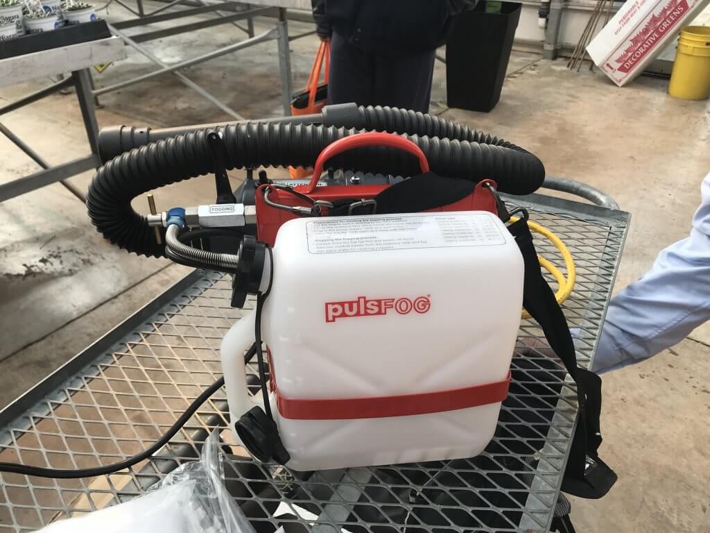
    When fogging, aim between the plants, such as the alleys and between hanging plants. This allows the fog to expand and permeate canopies for the best coverage. When spraying is done, be sure to release the pressure created in the spray tank to prevent accidental back flow into the gasoline tank.

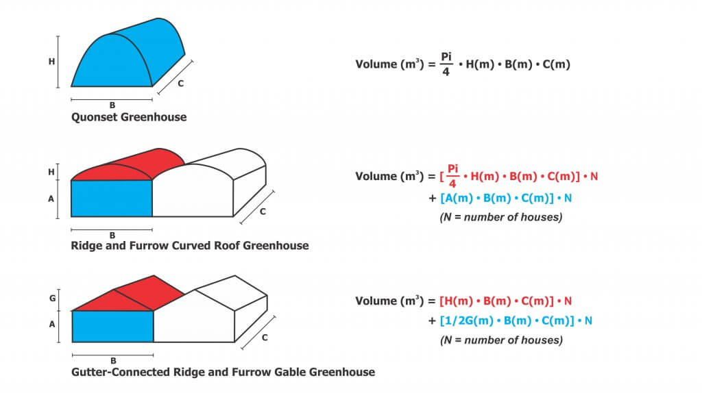
    And, because it’s convenient to include the math in this article, here are the formulae for calculating greenhouse volume to help you determine rates.
    Care and Maintenance

    HV, LV and ULV equipment requires model-specific cleaning and maintenance, according to manufacturer’s instructions. Even when sprayers are kept in prime condition, they are only as good as the operator’s understanding. When the wrong product is applied by the wrong machine using the wrong method, operators risk poor control, crop damage and increased potential for pesticide resistance. For more information, read the instructions that came with your sprayer, or contact the manufacturer.

    Thanks to Louis Damm and Dr. Heping Zhu for their contributions to this article.

    Try our calibration calculator: