Author: Jason Deveau

  • The Carvalho Boom and the Stages of Quadcopter Flight

    The Carvalho Boom and the Stages of Quadcopter Flight

    The Hypothesis

    The results of a recent herbicide deposition study performed with the DJI T100 led us to observe that after ~13 m/s, swath width and drift were no longer directly related to travel speed; They appeared unaffected. The result was completely unexpected as it was counter to several years of prior study with smaller drones. This led to a hypothesis that the aerodynamics of this new generation of quadcopters might be similar to that of a helicopter, and it was impacting spray deposition in a similar fashion.

    Let’s use the stages of quadcopter flight to set up the premise.

    1. Hover

    When a drone hovers, each rotor draws air from above and accelerates it downward in a high-velocity blast. The cumulative effect is a vertical component referred to as the “downwash” and the turbulent splash of air that hits the ground and spreads laterally is the “outwash”.
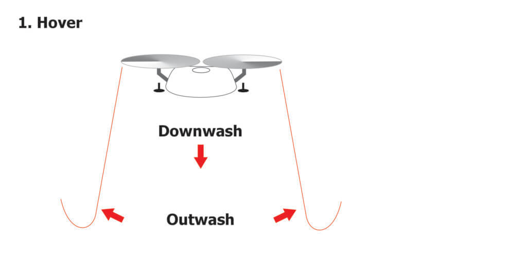
    The initial strength of the downwash depends on the degree of “disc loading” which is the weight of the drone divided by the rotor area. The intensity of the downwash wanes with distance from the rotor, spreading out in three dimensions until it impacts the ground and becomes the outwash.

    During hover, the drone recycles some of its downwash. This turbulence affects the stability of the drone, requiring a great deal of power to stay aloft, especially when it’s full.

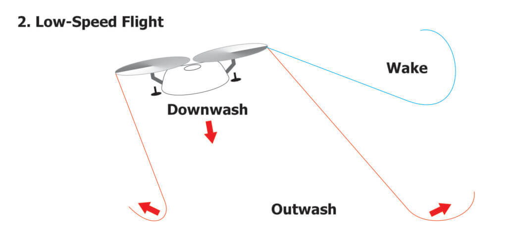
    2. Low-speed flight

    A helicopter achieves forward thrust by changing the pitch of its rotor blades. Most drones have fixed-pitch rotors, so the entire drone must tilt forward to enter low-speed flight. This causes the column of downwash to tilt backward.

    While the downwash is created by lift, “wake turbulence” is created at the tips of the rotors as high-pressure air beneath the rotor wraps around to the low-pressure area above. As the drone flies at low speed (~<3 m/s) the wake is visualized by a pair of counter-rotating, cylindrical vortices that trail behind. Some journal articles suggest the downwash for medium-sized drones (e.g. < 50 L capacity) detach from the ground at speeds as low as 3 m/s.
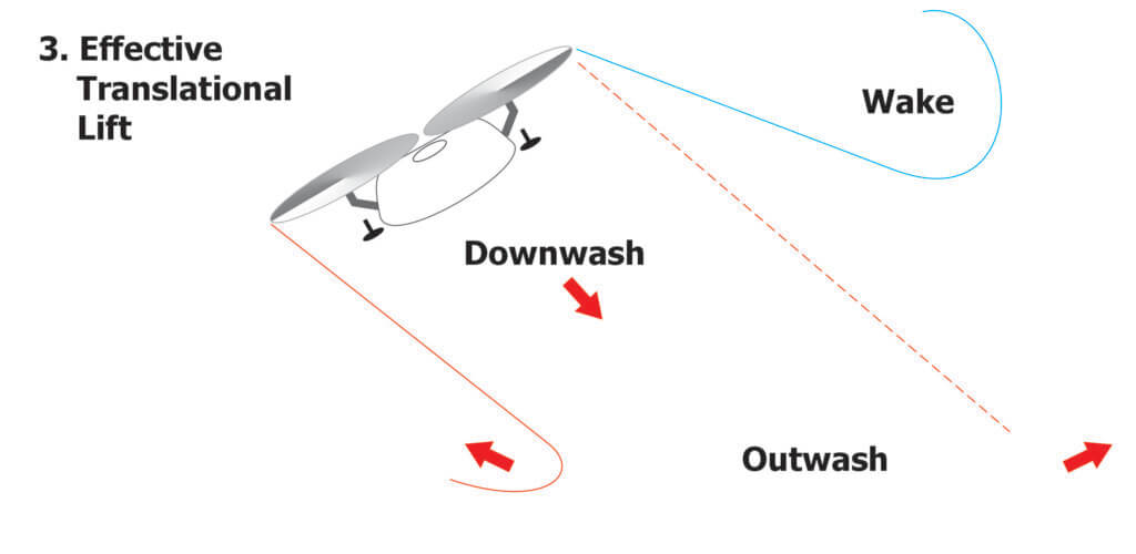
    3. Effective Translational Lift (EFT)

    As the drone accelerates it continues to angle forward, likely not exceeding 30°. At some point (~15 m/s?), we suggest it enters a state of “effective translational lift”, becoming more stable and therefore more energy efficient. This speed is notably slower than is commonly reported for a helicopter.

    During the transition, the drone behaves more like a wing as it essentially outruns its downwash, moving undisturbed air over the rotors. This horizontal air provides some lift, making flight more energy efficient, at least until drag begins to pull on the drone.
    The Possible Effect of Flight Stage on Spray Behaviour

    Droplets released beneath a drone at hover are completely entrained by the downwash. The majority get driven to the ground and then laterally along the outwash, while some small portion (likely smaller droplets) recirculate back up through the rotors.

    At low-speed flight, the downwash begins to tip backwards and the downwash trails behind and at some point detaches from the ground. Spray released beneath the drone is still entrained and will trail on a downward and rearward vector in that downwash. However, a portion will get caught in the wake. We can sometimes see this spray separation occur when lighting conditions are just right.

    As speed continues to increase, much of the spray would still be entrained in the downwash, but a greater portion would get caught in the wake, appearing as spray curling at the extremes of the swath. At some point, perhaps if and when the drone enters EFT, the the downwash might be less chaotic and behave more like laminar air. In which case some spray would still curl in the wake, but much of it would fall in a more stable sheet. Further increases in speed would not affect spray behaviour appreciably.

    Taking Advantage of ETL

    If this is the case, it is conceivable that rotary atomizers positioned under the front rotors could fling some droplets beyond the leading edge of the downwash. What if instead, it were a horizontal boom positioned out in front of the rotors, transecting the chord line?

    As the drone tipped forward during high-speed flight, so too would the boom, bringing it closer to the ground and releasing droplets ahead of, and below, the leading edge of the downwash. This should produce a more uniform swath, perhaps subsequently pushed down as the drone passed over.
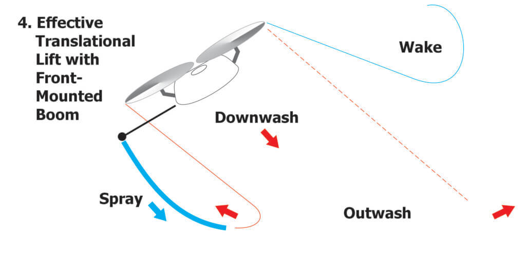
    It’s an interesting idea that is only made possible when drones are capable of high-speed flight.

    Reception

    In January 2026 I presented this concept during a lecture at the 4th annual Drone End-User meeting in Kansas City. The response was polite, but skeptical. I then shopped the idea around the trade show floor where drone manufacturers suggested a front-mounted boom would interfere with obstacle avoidance sensors, or shift the centre of gravity, making the drone difficult to fly and to land. And what about the impact of wind speed and direction? All good points. Then, Nino Carvalho introduced himself.

    The Carvalho Boom

    Nino Carvalho and his son, Emilio, own and operate NC Ag Spraying in the Central Valley of California, USA. Emilio was inspired to modify his drone after discussing matters with his mentors; one who owns and operates a fixed wing aerial business, and another that pilots a Huey helicopter. In late 2025, they designed and built a horizontal boom which I’ve dubbed “The Carvalho Boom”.

    Their first attempt was with a DJI T50, but the boom mount interfered with the stacked rotors, and the atomizer cables were difficult to extend. The XAG P150 had fewer cables and only top-mounted rotors, so it was a better fit. After experimenting with various materials (PVC was too flimsy, steel too heavy) they mounted a length of ½ inch metal conduit directly under the drone.

    In California, aircraft booms must be limited to 90% of the rotor width (because of rotor tip vortices). The greatest span of the rotors was 312 cm (122.8 in), so they made the boom 275 cm (~9 ft) long. They spaced the rotary atomizers evenly along the boom every 69 cm (~ 2 ft 3 in), extended the original 30.5 cm (12 in) nozzle cables to 305 cm (10 ft) to reach their respective electronic speed controllers, and plumbed them using 1.25 cm (0.5 in) diameter tubing.

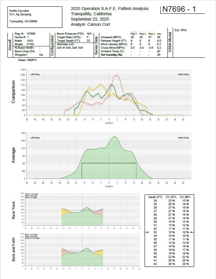
    They flew this first prototype over water sensitive papers. Dropping from a 3 m (10 ft) altitude to 2 m (6.6 ft) improved coverage uniformity and resulted in a 10.3 m (34 ft) effective swath width. They could see the downwash was interfering with deposition, and while increasing to a larger droplet size helped, it didn’t help enough. Then they made some design changes, extending the boom 30.5 cm (12 in) beyond the rotors, and they saw they had something. They reached out to Agri-Spray Consulting (Nebraska) and arranged to run a series of Operation S.A.F.E. fly-ins.
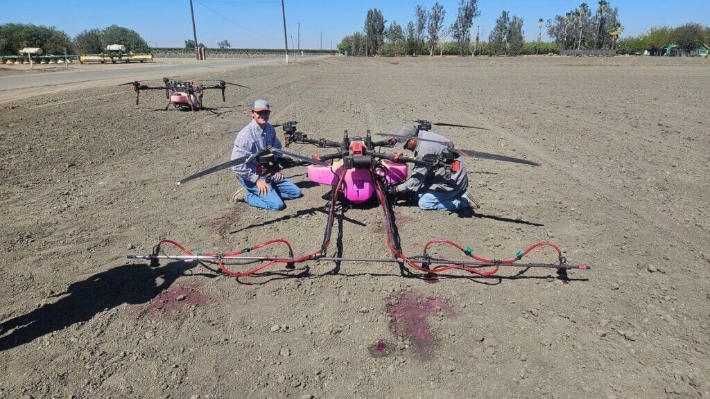
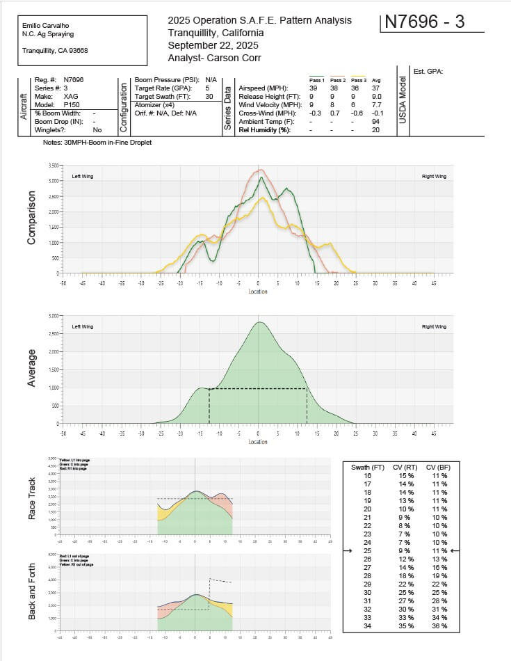
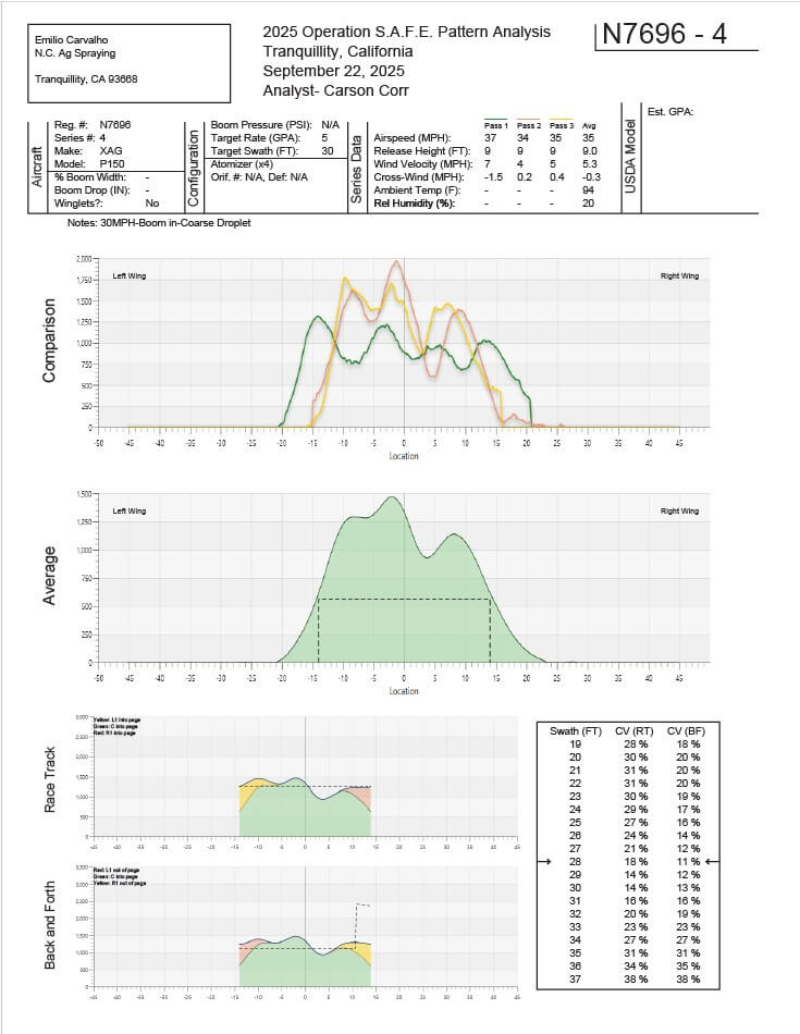
    There were more than 25 flights that day, so we’ll focus on three specific load-outs. The critical parameters are listed in the following table in the order that they flew them. The first load-out (N7696-01) was deemed the best, and was the only one with the boom extended out front, beyond the rotor tips. This information is italicized. The other two are included here for interest. N7696-03 attempted to shift the boom back under the drone for cosmetic reasons, but also for ease of transportation. N7696-04 was the same configuration as the last, but with coarser droplets in an attempt to battle the downwash. The first fly-in report (N7696-01) is shown below, but all three reports can be downloaded by clicking the links above.

    Load-OutBoom PositionVolume Speed Droplet Size (µm)Altitude Wind VelocityEffective Swath WidthC.V. (Race Track / Back & Forth)
    N7696-01Beyond Rotors50 L/ha
    (5 gpa)
    16 m/s
    (36 mph)
    2302.75 m
    (9 ft)
    10.7 kmh
    (6.7 mph)
    10 m
    (33 ft)
    10%/10%
    N7696-03Beneath Rotors50 L/ha
    (5 gpa)
    16.5 m/s
    (37 mph)
    2302.75 m
    (9 ft)
    12.5 kmh (7.7 mph)7.6 m
    (25 ft)
    9%/11%
    N7696-04Beneath Rotors50 L/ha
    (5 gpa)
    14.3 m/s
    (32 mph)
    4002.75 m
    (9 ft)
    8.5 kmh
    (5.3 mph)
    8.5 m
    (28 ft)
    18%/11%

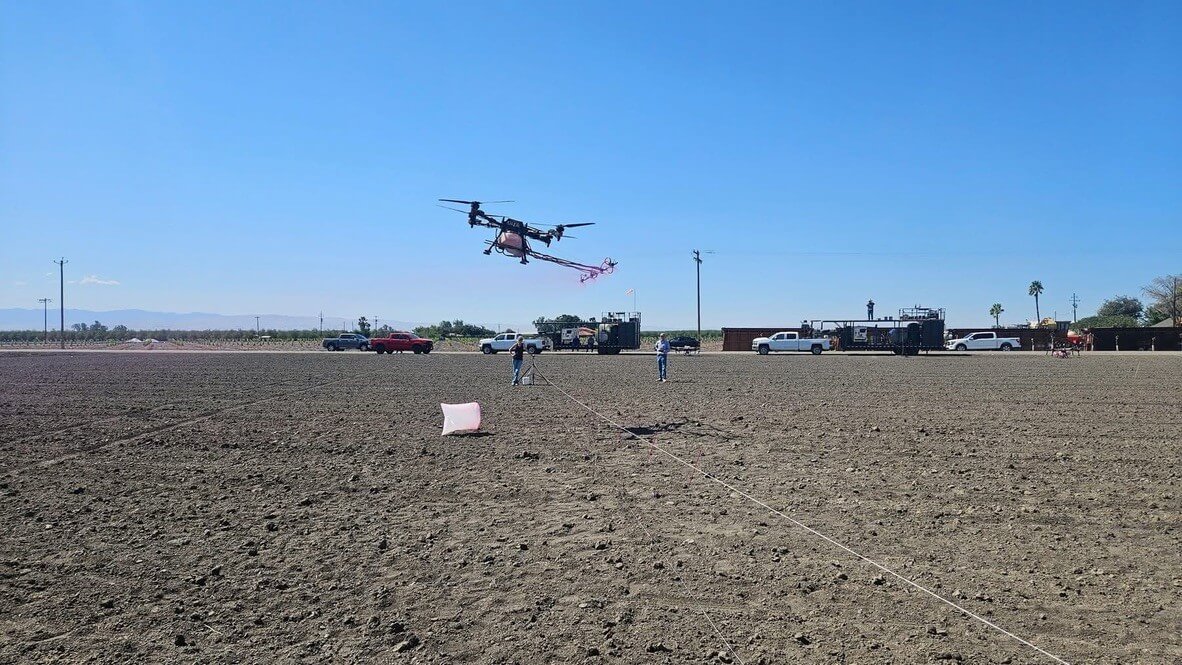
    Observers said it looked like the swath was rolled with a paintbrush and that there were no observable vortices – just a sheet of spray. The following videos show some of the passes from that day. Actually, you can see vortices, but only in the passes where the boom is positioned beneath the rotors and not when it’s extended out front.

    A 10% CV is spectacular, and the profile of each pass (even before averaging) was far flatter than any drone deposition I’ve seen previously. This design has not yet been used for custom application because there are still questions about how flight speed and pump flow will affect performance. But, the Carvalhos are already discussing the next design, constructed with carbon fibre tubes.

    Impacts and Musings

    Perhaps our description of how the air is moving over the drone is correct, or perhaps it isn’t quite right. Dr. Fernando Kassis Carvalho (no relation to Nino and Emilio) (AgroEfetiva, Sao Paulo, Brazil) recently shared that he also observed swath width no longer changed at speeds exceeding 13 or 14 m/s (personal communication). So, whatever the aerodynamic cause, the result seems clear.

    Does this mean we’ll see a new generation of quadcopters with front mounted booms? It’s certainly possible, and kind of poetic as some early drone designs featured a centrally-mounted boom that extended beyond the rotor tips. Emilio wondered aloud about possible wear on the front motors, and likely there will be other issues as they experiment, but it’s early days and they’re enthusiastic about pursuing the design.

    Nozzle Design

    Should we also consider a return to hydraulic nozzles? The rotary atomizers on a drone currently leave a lot to be desired. Dr. Ulisses Antuniassi (Prof., Sao Paulo State University) studied the spray quality produced by rotary atomizers. He ran atomizers from a DJI T40 and from a XAG P60 in a wind tunnel spraying WG and SL formulations with either MSO or NIS adjuvants and found no logical trends in VMD, relative span or DV 0.1

    Further, work by Dr. Steven Fredericks (Land O’Lakes) showed that the rotary atomizer from a DJI T40 created droplets roughly one ASABE category smaller than the software indicated. Conversely, common knowledge is that the XAG P100 version produces a coarser spray quality than anticipated, and slow motion video produced by Mark Ledebuhr (Application Insight LLC) and Dr. Michael Reinke (Michigan State University) clearly showed the flooding issue reported by Dr. Andrew Hewitt (University of Queensland), where excessive flow to the disc interferes with its ability produce a uniform droplet size.

    I photographed no less than nine different rotary atomizer designs while at the End-User meeting. So, perhaps we should embrace a standardized design, or perhaps hydraulic nozzles should make a comeback. If the later, it would be a great opportunity to include PWM to increase their flow range.

    Acceleration and Flight Pattern

    And what of kinematics? A drone’s “acceleration time” is calculated by dividing the change in velocity by the acceleration rate. We’ve seen that a DJI T100 must travel up to 100 m before it reaches target velocity. Admittedly, it was full and attempting to fly at high speed. Kevin Falk (Corteva Agriscience) noted a 25 m acceleration distance and a 15 m deceleration distance for a T50 flying mostly-full at 6 m/s. That’s a not-insignificant distance to achieve target flight speed.

    What happens to the spray from a quadcopter drone with a front mounted boom as it transitions through the stages of flight? We don’t know for sure, but we can infer an inconsistent swath. Perhaps the prolonged acceleration time is sufficient reason for drones to start flying racetrack flight patterns like planes and helicopters, where they reach sufficient speed before passing over and spraying the target area. Current software does not allow that practice.

    All this to say that as drone design continues to evolve, we must continue to challenge and test assumptions surrounding best practices. It has been fascinating to see how spray drones are finding their place in Western crop protection systems.

    Acknowledgements

    Thanks to Mark Ledebuhr (Application Insight LLC), Dr. Michael Reinke (Michigan State University), Kevin Falk (Corteva Agriscience), Dr. Tom Wolf (Application Research & Training), Adrian Rivard (Drone Spray Canada), and Adam Pfeffer (Bayer Crop Science) for insightful discussions.

    Special thanks to Nino and Emilio Carvalho (NC Ag Spraying) for sharing their experience and practical approach to improving drone spray deposition.

    Additional Resource

    In early February, 2026, I gave a short interview with RealAgriculture. We discussed the state of spray application by drone in Canada as well as some of the possible impacts of higher speeds.
  • Wanted: A New Technology for Assessing Spray Coverage – The Spray Doctor

    Wanted: A New Technology for Assessing Spray Coverage – The Spray Doctor

    “If you can’t measure it, you can’t improve it”. While the source is nebulous (Peter Drucker, Lord Kelvin, or Antoine-Augustin Cournot), the sentiment is clear.

    The status quo

    In the world of crop protection, considerable resources are expended to distribute a pesticide over a target. And yet, sprayer operational settings and spray coverage are rarely assessed. As a result, too much time elapses between the application and observing the biological results to evaluate and correct equipment performance. The damage (be it waste or an inconsistent and sub-lethal dose) is done. All sprayer operators know this to be true, so why do precious few perform these assessments?

    Perhaps, dear reader, you have personal experience assessing coverage and already know the answer. Perhaps you’ve performed the iterative dance that is placing, spraying, retrieving, assessing and re-placing water sensitive paper (WSP). Perhaps you’ve sprayed fluorescent tracers and hunted for faint glows at twilight using UV lights. Perhaps you’ve looked for residue from diatomaceous earth or fungicides. Or, perhaps, you’ve trusted in the falsely-comforting “shoulder check” and assumed dripping must mean you’ve hit the target.

    Existing methods are complicated, subjective, messy and time-consuming. We need an alternative.

    The alternative

    Consider a permanent, solar-powered sensor that supplies real-time spray coverage data to your smartphone via a cellular connection. The output could be visualised in a simple and intuitive way, and immediately available to both sprayer operators and farm managers. If the sensor was relatively inexpensive, sufficiently hardy, and easy to deploy, its utility would only be limited by your imagination:

    • Stakeholders could confirm the correct functioning of their equipment before committing to the application. Decisions could be made to change operational settings, repair equipment, or delay until conditions improved.
    • The sensors would provide coverage data specific to their location and orientation. Units could be installed in difficult-to-spray regions such as treetops, or canopy-centres, or fruiting zones. Sensors could be placed where pest/disease pressure has been historically high, or where wind is a known issue.
    • Large operations could install them in a test-row, where sprayer operators would perform a gauntlet-style calibration run prior to a day of spraying.
    • Spray records could inform compliance audits, supplement insurance or CanadaGAP traceability requirements, or be used in agronomic assessments.

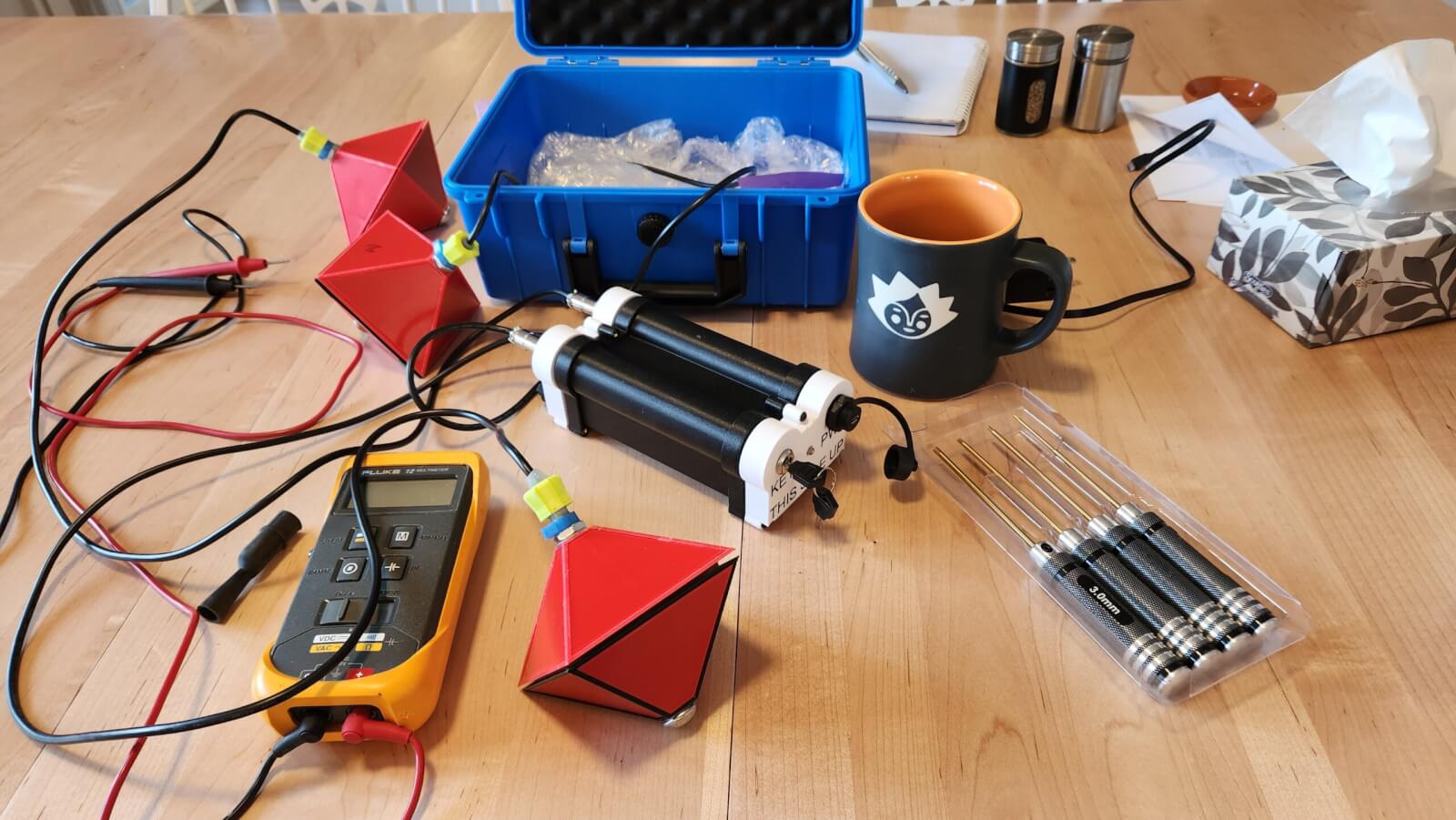
    In 2025 I was approached by an Australian developer who claimed he had a device that did all of this. And, if that weren’t enough, it could also monitor certain meteorological factors such as pre-spray moisture levels and temperature and report post-spray evaporation rates. I could barely contain my excitement. A prototype was in my hands a few weeks later.

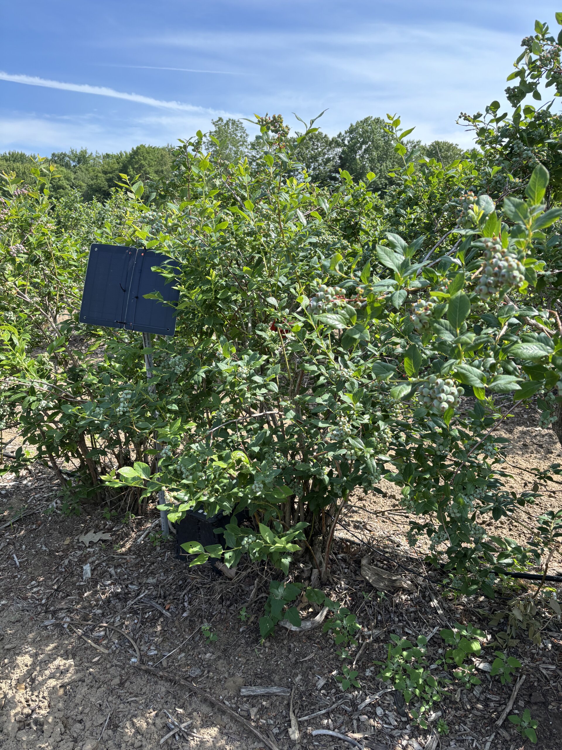
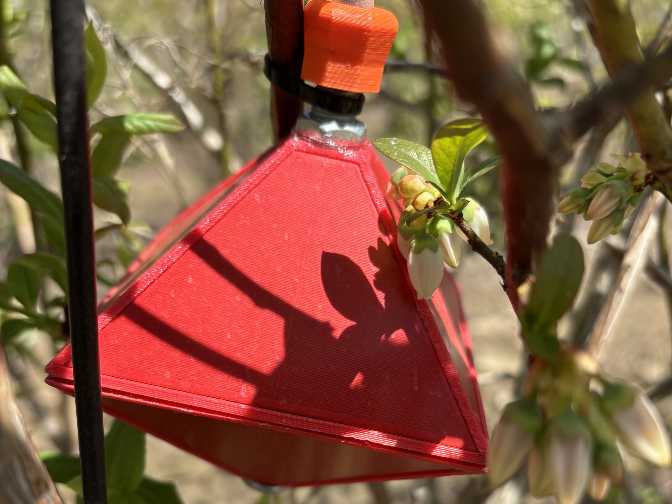
    Prototype, 8-sided sensor located in a blueberry bush.
    Solar panel powering three, 8-sided prototype sensors spanning 10 meters of highbush blueberry.

    Benchmarking the sensor

    The Spray Doctor (working name for the prototype) started its life as a leaf wetness sensor, evolving into a spray coverage sensor piloted in 2023/24 in Australian and New Zealand grape production. The history of earlier iterations and company schisms is convoluted, and fortunately immaterial to our purposes. All I needed to know was that we weren’t starting from scratch. Several of the questions regarding how accurately the surface could detect spray deposition were already addressed by independent research.

    The sensing surface is impregnated with an array of capacitive wetness sensors. The sensor responds to the surface area covered and not deposit density. Researchers reported a reliable response range between ~10% and 50% surface coverage. Given the arguable “ideal” coverage standard of 10-15% surface area, this includes the range of interest for most sprays.

    Benchmarking against WSP was part of the foundational assessment. A droplet of water deposited on WSP produces a high angle of contact and very little spread, while the same droplet deposited on plant tissue tends to produce a lower angle of contact and more spread. This means the stain produced on WSP is smaller than would be produced on plant tissue, depending on how smooth, vertical or waxy the tissue surface was.

    It was therefore surprising that WSP were found to report a higher degree of spray coverage during water-only sprays than the sensor. It seemed droplets more easily coalesced and ran off the sensor surface. This was ultimately interpreted as an advantage, because the sensor would better emulate how a leaf surface would respond to the influence of surfactants and spray quality.

    Adding a surfactant to a spray solution improves droplet adherence, and/or reduces surface tension, improving the degree of contact on plant surfaces. Likewise, it was found that surfactants increased the degree of coverage reported by the sensor, and when actual chemistry was sprayed (e.g. sulphur powder or copper sulfate) there was an effect on the degree of coverage reported. This is unlike WSP, where adjuvants and chemistry do little to increase the spread.

    And so, like every method for assessing spray coverage, the sensor has limitations and caveats. If you have some doubt as to the sensor’s accuracy, do not get distracted by the fine detail. Remember, most operators currently have no feedback whatsoever; even a binary response (e.g. hit or miss) would be welcome. The sensor is sufficiently sensitive and consistent to resolve coverage in a range relevant to most sprays, and therefore worth field testing.

    The experiment

    My role in this story was to work with a grower to evaluate the sensor’s ability to report coverage information in a clear and actionable way. There were three questions:

    • Does data from the sensor influence a sprayer operator’s behaviour?
    • Does that change in behaviour lead to improved spray coverage (implying more efficient and effective crop protection).
    • Could we “dial in” the hardware and the interface based on the grower’s feedback?

    In part two, we share our experience installing and using the Spray Doctor, as well as supply answers to these questions. Stay tuned.

    Thanks to Brandon Falcon (Falcon Blueberries) for volunteering his time and farm for this evaluation, and the developer for the in kind donation of the prototype Spray Doctor.

  • The Micothon M2 – The Benefit of Air-assist Spraying in a Vegetable Greenhouse

    The Micothon M2 – The Benefit of Air-assist Spraying in a Vegetable Greenhouse

    I’ve experienced a few spectacular failures trying to build niche sprayers. Until now, I haven’t had a reason to write much about them. But I decided the contrast, and confession, would be a fun way to set the scene for a discussion about an excellent niche sprayer.

    Failed Attempts

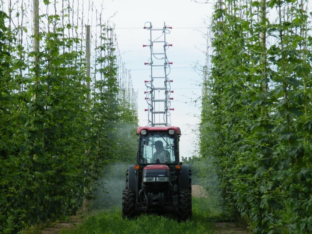
    First, the ill-fated “Hops Sprayer”. We used an adjustable ladder to position 20 feet of arborist guns between hop rows. The nozzles could be raised and engaged to match the growing crop canopy. While it left decent coverage on the adaxial surfaces, we quickly realized it needed air-assist to get under the leaves and battle high winds at the top of the trellis. It’s since been cannibalized for parts, and the rusted remains haunt me whenever I drive by the outdoor storage area at our ag research station.

    The Hops Sprayer. A 3 point hitch, vertical boom that could adapt to match canopy height.

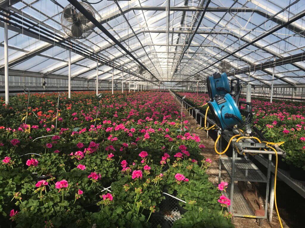
    Later, encouraged by a minor success ducting a backpack mist blower with PVC and Coroplast, I tried building an air-assisted spray cart for a floriculture operation. It featured commercial, high-volume radial fans paired with hollow cone nozzles positioned in front of the air outlets. With respect to GreenTech and Croplands Equipment in Australia, I tried to build a bargain-basement SARDI-style head.

    When it wasn’t threatening to tip over, it managed decent coverage over almost 2 meters. Almost.

    As it turns out there’s a very good reason engineers use computational fluid dynamics to design air-assisted sprayers. We were ultimately beaten by an uneven greenhouse floor crowded with obstacles, a stiff canopy of geraniums, and the inverse square law, which states: “The farther away an object is from an effect, the less change can be observed in the object”. This rig now has a new life circulating hot air in a boiler room.

    And I once built an air-assisted, tow-behind sprayer to spray troughs of tabletop, hoop house strawberries. That unit laid down an excellent, uniform spray on all foliar surfaces, but it was frustrating to use. There was almost no clearance in the hoop house, which changed height with the topography, and the alternator couldn’t keep the battery sufficiently charged to run the pump and fans. I felt we could overcome these small difficulties, but sadly the operator ended this experiment halfway through the season. I can only assume the sprayer is now an interesting piece of lawn sculpture.

    This sprayer had potential, but limited resources prevented it from getting beyond the beta stage.

    The Micothon M2

    Despite my inability to build a decent air-assisted sprayer, I have always maintained that air-assist is the secret sauce for efficient, uniform spray coverage. Lucky for me, Great Lakes Greenhouses (GLG) agreed. No stranger to innovation, the company recently purchased a first generation, air-assisted Micothon M2 greenhouse sprayer and invited me to come see it. This was a proper sprayer designed by engineers, and not a delusional plant physiologist, so I was excited to assess and calibrate it. This article will describe what we learned and perhaps in some small way, validate my failed attempts.

    A quick walk around before we got to spraying.

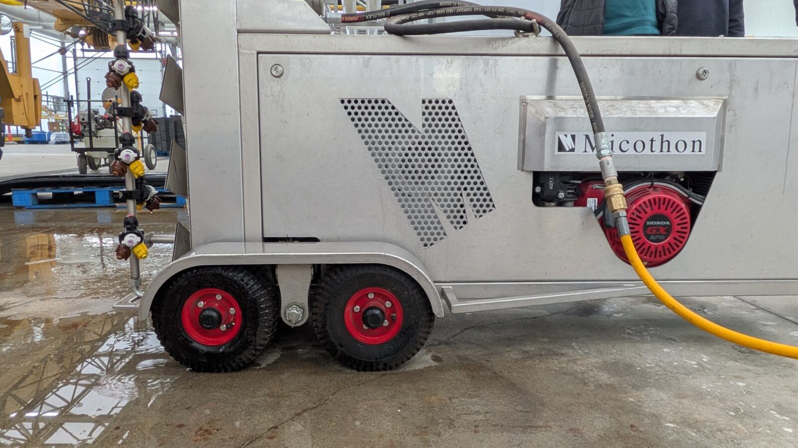
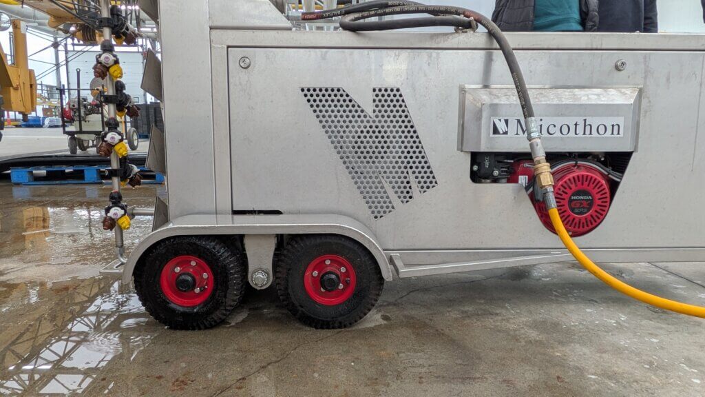
    The M2 features a vertical boom design supported by a portable tender unit, but that’s where the similarities to a classic “tree” sprayer end. Rather than riding on the hot water pipes, or tipping onto two wheels like a hand cart, this version rides on self-leveling wheels. It is drive-assisted but still has to be guided by an operator, like a self-propelled walk-behind lawn mower.

    Drive-assist, self-levelling wheels.

    The mast features 18, three-position nozzle turrets (nine to a side). GLG requested a bespoke spring-loaded break-away section at the top of the boom. This allowed the top nozzles to “duck” under an annoying section of greenhouse infrastructure that would have otherwise prevented it from being positioned between the rows.

    A spring-loaded, break-away boom section (with guard) to prevent impact damage.
    The break-away section in action.

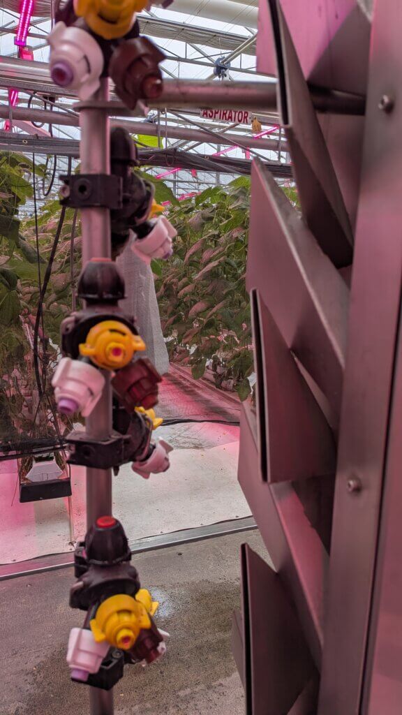
    The air is generated by a centrifugal fan powered by a Honda motor. The air travels up the ducted mast to a manifold of narrow air outlets. When the sprayer is moving, the air outlets precede the nozzles, which initially seemed wrong as the spray would be released outside the air stream. But, upon closer inspection, we saw that the air outlets are not only angled up by 45 degrees but are also angled back so the air can transect the spray.

    Air outlets and nozzles – front view.
    Air outlets and nozzles – side view.

    It was suggested that the blade of air acts like an airfoil, creating an area of low pressure and sucking small droplets into the airstream. This is Bernoulli’s principle and it describes how wings create lift. Personally, I think it behaved more like a Venturi. I’m open to debate since, as evidenced by my attempts at building a sprayer, I’m no engineer. What matters is that we didn’t see any droplets hanging in the air as the sprayer passed. It works.

    Calibration and Optimization

    We followed the same greenhouse sprayer optimization protocol I’ve outlined in this article. Go give it a quick read and come back so I won’t have to reiterate why we took the steps we did.

    Travel speed and air settings

    The sprayer was set to speed “3” of a possible “5”, as recommended by Micothon. Travel speed dictates dwell time, which is the duration the air is focused on the target. Observers stood in the drive alley and in the two adjacent alleys to see how the air moved leaves. The upward angle of the outlets combined with the volume produced by the centrifugal fan wafted and twisted leaves on their petioles. This created sufficient movement throughout the canopy, but not so much that it caused the canopy to louver shut. It was a Goldilocks situation so there was no need to alter anything.

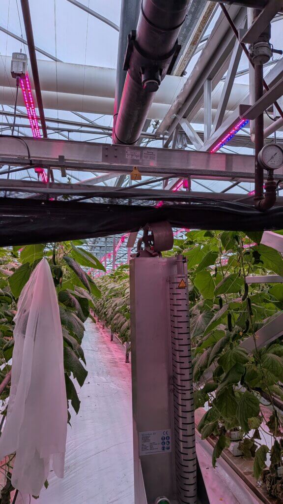
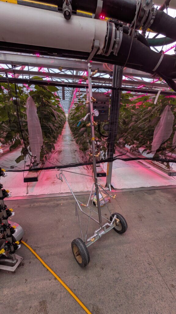
    Preparing to guide the Micothon M2 through the cucumbers under red LED lights. This image gives perspective of canopy height, density and the sprayer clearance.

    Pressure and nozzles

    The tender system regulator was set to 41.5 bar (600 psi) and that pressure dropped to 5.5 bar (80 psi) according to the gauge on the sprayer. While we didn’t test it, I’m certain the pressure at the furthest (aka highest) nozzle would have been closer to 5 bar (~70 psi). With observers in place, we started spraying water using the Albuz 025 (lilac) hollow cone tips.

    We saw the highest nozzle positions were spraying over the canopies and did not need to be on. We also saw drip points form at the tips of the leaves and the bottom of the cucumbers. There was evidence of yellowed (possibly damaged) tissue at the leaf tips, suggesting they were often sprayed to drip. This is wasteful and tends to redistribute deposits in undesirable ways. While it’s hard to avoid on the waxy, vertical cucumbers, it can be prevented on the leaves.

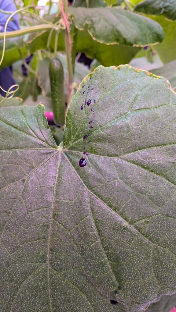
    Note the drip point formed at the bottom of the fruit. This is hard to avoid, but can at least be minimized.

    We turned off the top nozzles, swapped to Albuz 02 (yellow) hollow cones, moved to an unsprayed canopy and tried again. Effectively this was a 20% cut in water and product, but there were no more drips on leaves and less evidence of coalescing deposits. The cucumbers still had drip points, but without an adjuvant that was the best we could do. That’s assuming there would be value in spraying the fruit in the first place – these sprays were targeting the foliage.

    Coverage

    With the subjective part of the assessment complete, it was time to quantify spray coverage. Water sensitive papers were oriented co-planar with the leaves and essentially parallel to the ground. We clipped them 2-3 cm below the leaves by affixing them to the petioles. This way they would move with the leaf and represent a very challenging target (reminiscent of a sucking insect on the abaxial leaf surface).

    This is a difficult target to hit. The spray must get up between the leaf and upper side of the water sensitive paper, which is not in line-of-sight of the nozzle.

    We divided the canopy into quarters, placing one target in each section. This spanned the height of the canopy, but we also positioned them along the canopy depth: One on each of the four plants in the row. This left us with a diagonal cross-section. Read it again – you’ll get it.

    Then we sprayed the row from one side and inspected the results. We saw excellent coverage on the abaxial surfaces of the two plants closest to the sprayer. We expected that. But we were pleasantly surprised to see the spray got in under the umbrella-like leaves and deposited on the adaxial surfaces. This was not line-of-sight for the nozzles, and there wasn’t much room between the paper and the underside of the leaves, so this was clearly the result of air-assisted droplets.

    There was also respectable coverage on the two plants on the far side of the row. These targets were greatly improved once we travelled down that alley and saw the cumulative coverage. This is why you should (almost) never perform alternate row spraying.

    Abaxial side of the water sensitive papers. From left to right, papers ascended from the lower quarter of the nearest plant to the upper quarter of the farthest plant in the row.
    Adaxial side of the water sensitive papers. From left to right, papers ascended from the lower quarter of the nearest plant to the upper quarter of the farthest plant in the row.

    Compared to a tree

    Since I was in the neighbourhood, we decided to see what a conventional, hydraulic tree could do by way of comparison. Frankly, there was none.

    A typical greenhouse tree. Note the 1/4 turn drain near the pressure gauge, the lack of check valves, and the uneven distribution of the nozzle positions (i.e. more at the top) likely intended to direct more flow higher in the canopy.

    The tree was nozzled with Albuz 04 (red) hollow cones angled upwards. There were only a few check valves, so it leaked when it was turned off and had to be drained at the end of each row using a quarter turn valve. Coverage was generally excessive (i.e. coalesced droplets and lots of run-off) and non-uniform (we randomly missed both adaxial and abaxial surfaces).

    Run-off was so pronounced that it washed the dye off the water sensitive papers.

    We re-nozzled to my favourite load out: TeeJet TwinJet fans alternating back and forth by 45 degrees from centre. Using 03’s (blue), we observed improved uniformity, but still saw misses and suspected we were still using too much water. When leaves are drenched they get heavy, causing them to hang lower and obscure the other parts of the plant. This is the contradiction that limits a strictly hydraulic system: Pressure motivates droplet movement, so you need slightly larger drops and more volume. However, too much water causes run-off and weighs leaves down, obscuring the rest of the canopy. Catch 22.

    I proposed getting a set of 02 (yellow) tips in the hopes there would still be enough spray for better uniformity. I hope they tried it.

    A few beefs about the M2

    There’s always room for improvement. Before you think I’m selling these sprayers, here are a few observations from the owners and from what we saw that day. No deal breakers, just some nice-to-haves:

    • The diesel exhaust from both the sprayer and the tender cart is not ideal. Applicators wear respirators, and the greenhouse fans tend to dilute the exhaust, but a battery system (perhaps like a drone) would be preferable to power the drive electrically.
    • There was a latency with the self-leveling wheels and with air build-up in the tower portion of the sprayer. You simply need to be patient before you start down a row.
    • The tower section gets hot to the touch, likely because of the position of the exhaust pipe.
    • The alternator on board recharges the battery, but if you let it sit the battery is depleted (sounds like the same trouble I had with my sprayer, which is somehow gratifying).

    I’m sure you’re asking “How much?”

    Well, at the time of writing, it was almost $70,000.00 CDN, but don’t judge it too harshly! Bear in mind that our assessment saw a reduction of 20% water and crop protection product that would otherwise have ended up on the greenhouse floor. Not only is that a big savings in water and inputs, but it’s fewer refills and it produced far better spray coverage that a hydraulic system. While improved coverage is not always linked to improved efficacy, they certainly go hand in hand. And when we’re considering “softer”, biorational greenhouse chemistries, improved coverage is the best bet we have for pest control.

    All in all, this was an excellent sprayer that I hope is the first of many to grace Ontario’s greenhouses.

    Thanks to Great Lakes Greenhouses for the invitation, and thanks to all the other grower cooperators (names withheld to protect the innocent) that took a risk on building budget, niche sprayers with me. Sometimes, you just have to throw money at it.

  • Canada Gazette Part II – Recent and upcoming changes to Canadian rules for operating RPAS

    Canada Gazette Part II – Recent and upcoming changes to Canadian rules for operating RPAS

    Editor’s Note: This article was posted in June 2025, and as of November 4, 2025, the rules described in this article have now come into effect. Further, on June 30, 2026, Health Canada published Science Policy Document SPN2026-02, allowing pesticide application by remotely piloted aircraft systems (RPAS; commonly known as drones) for products currently registered for aerial application. Each province and territory is currently updating policy in response to this document, so be certain to understand and comply with regional rules and regulations before using RPAS to apply pesticides. A more recent article can be found here.

    Summary

    The Government of Canada introduced the first set of Remote Piloted Aerial Systems (RPAS) rules in 2019, which addressed safety concerns and created a flexible and predictable environment for small RPAS flown within visual line-of-sight (VLOS). On March 6, 2025, amendments were made to the Canadian Aviation Regulations (RPAS – Beyond Visual Line-of-Sight and Other Operations): SOR/2025-70 Canada Gazette, Part II, Volume 159, Number 7. According to the Impact Analysis Statement in the document, the changes:

    • permit RPAS <150 kg to be flown within visual line-of-sight;
    • introduce rules for routine beyond visual line-of-sight (BVLOS) operations for RPAS <150 kg
      • over sparsely populated areas,
      • at low altitudes, and
      • in uncontrolled airspace;
    • remove the requirement for a Special Flight Operations Certificate (SFOC) for these operations;
    • include requirements for
      • new pilot certification,
      • new technical standards for the aircraft and supporting systems,
      • new operational procedures, such as increased distances from airports, heliports, and people, as well as
      • new requirements for individuals and organizations to operate BVLOS.

    In addition, the Regulations will update existing service fees and introduce fees for existing services that are currently provided for free and the new services that will be provided to the RPAS sector.

    These regulatory changes are driven by agriculture, but also increasing utility in package delivery, use in emergency response (e.g. fire assessment), environmental impact assessment and infrastructure inspection.

    The original document is lengthy, so only those changes that relate to the use of spray drones are reproduced here. For more details, refer to the Regulations Amending the Canadian Aviation Regulations (RPAS – Beyond Visual Line-of-Sight and Other Operations) Canada Gazette, Part II, Volume 159, Number 7. Transport Canada has a summary of the changes here.

    At the time of writing, there are no agricultural, terrestrial pesticides registered for application by RPAS in Canada. Health Canada’s Pesticide Compliance Program (PCP) is responsible for promoting, monitoring and enforcing the Pest Control Products Act (PCPA). Their factsheet can be downloaded here.

    Objectives

    There are three objectives to the new regulations:

    • Regulatory predictability, economic growth, and innovation
    • Safety risk mitigation
    • Fee modernization

    The regulations build upon Part IX of the CARs and introduce new requirements to reflect the increased risks of the two new categories of operation:

    • Medium drones that weigh above 25 kg up to and including 150 kg flying within VLOS near and over people, in both controlled and uncontrolled airspace; and
    • Drones that weigh 250 g up to and including 150 kg flying BVLOS in unpopulated and sparsely populated areas, below 400 feet above ground level, and in uncontrolled airspace.

    Grouping the new regulations – The 3 P’s

    The new regulations can be grouped into:

    • Pilot (pilot training and certification)
    • Product (aircraft and supporting systems)
    • Procedures (operational rules)

    In addition, there are new requirements for individuals and organizations operating BVLOS, such as appointing an accountable executive, and requirements to establish training programs and risk management processes, which are discussed in more detail below. These new requirements will allow for clearer organizational oversight with larger-scale operations, covering larger geographic areas, as well as an increase in the number and types of drones being operated.

    The Pilot

    Advanced Pilot Certificate

    TC has determined that the following operations may be added to the types of operations conducted by Advanced Pilot Certificate holders, without the requirement to obtain a new pilot certificate:

    • VLOS operations with a medium-sized drone (above 25 kg up to and including 150 kg).
    • Extended VLOS operations (EVLOS), using a visual observer to scan the airspace.
    • Sheltered operations, which allow the drone to be flown around a building or structure without the use of a visual observer.

    Advanced Pilot Certificate operators will be required to pay fees associated with the obtaining the certificate:

    • $10 exam fee, paid to the Government of Canada (GoF).
    • $25 certificate issuance fee, paid to the GoC.
    • $257 flight review fee, paid to the flight reviewer.

    Pilot Certificate for Level 1 Complex Operations (Lower-risk BVLOS)

    The Regulations will introduce a new pilot certification process for lower-risk BVLOS called Level 1 Complex Operations. A pilot must be at least 18 years old and have their Advanced operations certification.

    • Pilot must attend RPAS training (“ground school”).
    • Pilot will need to pass a new online multiple-choice exam delivered through TC’s DMP.
    • Pilot will need to visit a flight reviewer to do an in-person flight review.

    Every two years, pilots will need to do at least one training renewal activity recognized by TC (e.g. flight review, training activities, or retaking one of the pilot exams in the DMP.)

    CARs 901.19, Fitness of Crew Members, and the requirements of the RPAS Operator Certificate (RPOC) provide sufficient mitigations to maintain safety within the level of risk for BVLOS operations. However, a medical standard for operations outside the lower-risk category may be considered in future regulatory work.

    Commercial RPAS operators will need to hold a Level 1 Complex Certificate to conduct lower-risk BVLOS operations. To receive their Level 1 Complex Certificate, operators will need to pay a certificate fee of $125 to TC.

    Advertised Events

    Part IX of the CARs requires operators of RPAS of at least 250 g to obtain an SFOC to operate at an advertised event, which is defined as “an outdoor event that is advertised to the general public, including a concert, festival, market or sporting event.” The Regulations will expand this requirement to all RPAS, including microdrones weighing less than 250 g.

    The Product

    Drone registration is expanded to all drones 250 g and above.

    Declaration

    A drone won’t be permitted to fly in an operating environment unless the manufacturer supplies a Declaration (online form, Standard 992) or a Pre-Validated Declaration (PVD) for that respective operating environment. Operating environments include medium-sized drone in controlled, or uncontrolled airspace, or away from people, or BVLOS operation away from populated areas below 400 ft and in uncontrolled airspace.

    The PVD is a two-step process where the plan for the aircraft design is submitted in the context of Standard 922, and when approved, then they complete the Declaration. Operating environments include VLOS with medium-sized drones near and over people, and certain BVLOS operations over sparsely populated areas, below 400 ft and in uncontrolled airspace.

    Maintaining a PVD requires annual reports of the estimated number of flight hours, a description of any safety-related issues, and any relevant design changes.

    The Procedures

    Advanced Pilot Certificate holders can perform Extended VLOS (EVLOS) operations and sheltered operations if:

    • The drone is within a certain distance from the pilot, while a second person with a Basic Pilot Certificate scans the airspace and notifies the pilot of any other airspace users or hazards.
    • Performing a sheltered operation, the pilot may fly their drone around a structure without keeping the drone in direct line-of-sight, if they keep the drone within a certain distance to the structure (intended for building inspections).
    • The Regulations increase the minimum distance from people not involved in the operation and require additional planning considerations such as weather conditions that could affect the pilot’s ability to maintain line-of-sight.

    Lower-risk BVLOS

    Pilots will need to remain in uncontrolled airspace away from aerodromes, below 400 feet, and over unpopulated or sparsely populated areas (i.e. <25 people/km2 per Stats Canada and the Drone Site Selection Tool.

    RPAS Operator Certificate (RPOC)

    The new RPOC focuses on risk management and addresses the trend of larger fleets, longer flight times and BVLOS operations. The RPOC is an assurance there are policies and procedures in place that reflect the size and complexity of the operations. It is a Declaration to TC that the pilot or organization meets requirements in CARs (via the DMP) and there is no requirement for renewal.

    Fees for services

    Basically, the RPAS Operator Certificate fee is $125 CDN with the goal to lower the cumulative cost of BVLOS. The SFOC structure, which originally proposed two steps (Low-Complexity and High-Complexity) now has two new categories: Very-Low and Medium Complexity. Fees were revised to reflect the different levels of complexity and the related levels of effort that would be required by TC. These fees will be adjusted for inflation.

    Fines (Administrative Monetary Penalties)

    Under the Aeronautics Act, the Minister of Transport has the authority to issue administrative monetary penalties (AMPs) to anyone who violates designated provisions of the Act and the CARs. Most of the provisions in Part IX of the CARs are enforced through the assessment of AMPs imposed in accordance with sections 7.6 to 8.2 of the Act, which carry a maximum fine of $5,000 for individuals and $25,000 for corporations and include the potential suspension or cancellation of a person’s Canadian Aviation Document.

    When do the new regulations come into force?

    New regulations will be introduced in stages to give stakeholders the opportunity to become certified and to familiarize themselves with the new requirements before the 2026 season. Some regulations will come into force on April 1, 2025, but others will activate when they are published in the Canada Gazette, Part II, including:

    • the ability to register drones
    • submit declarations and take new pilot exams

    The remaining provisions will come into force on November 4, 2025, such as:

    • provisions relating operating medium-sized drones in beyond visual line-of-sight (BVLOS) in lower-risk environments.

    For more information, see the Regulations Amending the Canadian Aviation Regulations (RPAS – Beyond Visual Line-of-Sight and Other Operations) Canada Gazette, Part II, Volume 159, Number 7.

    Also see this short-and-sweet summary from RealAgriculture.

  • Exploring the Accuracy of Drone-Applied Herbicide Treatments

    Exploring the Accuracy of Drone-Applied Herbicide Treatments

    Author’s note: Minor edits were made to this article since the original publication. While the results remain unchanged, aspects of the interpretation have been adjusted upon reflection.

    In 2024, Corteva conducted a study entitled “Drone-Delivered Herbicides: Comparing LontrelTM XC (Clopyralid) Efficacy Across Application Techniques and Water Volumes”. Go read all about it here. Their objective was to compare the relative efficacy of hand booms and drones, and to determine if drone efficacy was affected by low water rates. The researchers evaluated the area treated and the effective swath width by manually tracing the burned areas from an aerial NDVI image.

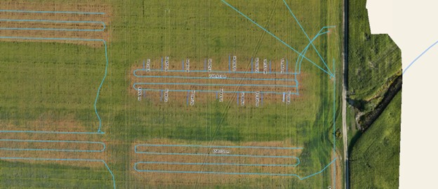
    Interestingly, the study found that water volume had an insignificant impact on herbicide efficacy. But what really caught our attention was the inconsistent and variable shape of the treated area along each flight path (Figure 1).

    Figure 1 – Image from work performed by Kevin Falk, Rory Degenhardt, Angela Fawcett and Neil Spomer, as presented at the 2025 Canadian Weed Science Society annual meeting in Vancouver, BC.

    If the swath width fluctuates and vacillates along the flight path, then there is great potential for overlaps and misses throughout a treated area. Common practice is to rely on displacement (and drift) from upwind passes to deposit a sufficient cumulative dose of herbicide to mask areas of low coverage. This would be facilitated by consistent wind direction, higher altitudes, and a surface with little or no canopy to interfere with secondary deposition.

    On the other hand, if the programmed swath width (i.e. route spacing) is too wide, and/or the the droplet size too large to permit sufficient displacement, then gaps in coverage would appear. And there is always the consideration of restricting the deposit to field boundaries and margins, particularly on the downwind side of the treatment area.

    We explored these considerations by conducting a study that emulated aspects of Corteva’s work. We applied Roundup Transorb HC (a non-selective herbicide) instead of Lontrel (a selective herbicide specifically for broadleaf weeds). We used the DJI Agras T50 and the new T100 with two atomizers and a DJI RTK-2 base station, employing an array of operational settings. And, we flew multiple passes rather than a single pass for each treatment.

    Part one of the study examined three programmed swath widths from both drones to compare their performances directly. Part two of the study evaluated the T100’s performance over a series of flight speeds and spray qualities. Burndown was evaluated using post-application orthomosaic images taken at 200 feet using a DJI M3M drone. Images were analyzed using Pix4D software.

    Materials and Methods

    Field Conditions

    Applications took place in a 160-acre field of wheat stubble in Central Elgin, Ontario (42°45’29.3″N 81°05’58.9″W) on September 13, 2025.

    Treatments

    Each flight was centred on the right boundary of the treatment block, as indicated by a pin flag. Four passes were flown per treatment (i.e. two out-and-backs). There were no repetitions for treatments, so there was no need to randomize them.

    Part One

    The intent of this part of the study was to make a direct comparison of the swaths produced by the T50 and the T100. The T100 is heavier, has a larger volumetric capacity (100 L vs. 40 L) and is capable of faster flight (20 m/s or 64 km/h vs, 10 m/s or 23 km/h). We wrote about our first impressions of the T100, here.

    Drone operational settings were selected to replicate those used in previous corn and wheat fungicide experiments with the T50. These settings are admittedly more restrictive (from the perspective of productivity) than those commonly used for herbicide applications. For example, and anecdotally, we have been told the T100 can spray a full section (~260 hectares or 640 acres) at 2.8 gpa and 20 m/s on one tank and one battery charge. However, we have no information about subsequent coverage, efficacy or off-target deposition.

    Maintaining these operational settings allowed us to make a more direct comparison of herbicide vs. fungicide placement and efficacy. All applications were performed using a 250 µm spray quality (Table 1).

    Treatment CodeRPASProgrammed Swath (m)Speed
    (m/s, km/h)
    Altitude (m)Volume (gpa)
    AUnsprayed––––
    BT5066, 21.635
    CT5086, 21.635
    DT50106, 21.635
    ET50610, 3635
    FT50810, 3635
    GT50108, 28.8*35
    HT10066, 21.635
    IT10086, 21.635
    JT100106, 21.635
    KT100610, 3635
    LT100810, 3635
    MT1001010, 36*35
    Table 1 – Part one: Drone settings. (*10 m/s was intended, but the T50’s pumps could not produce a 10 m swath at 5 gpa at that speed.)

    Each treatment block was 150 m long, 50 m wide and a 20 m buffer was maintained between treatments (Figure 2). Two, 1 m scale indicators were placed in Treatment B to confirm scale during image analysis.

    Figure 2 – Part one treatment layout.

    Part Two

    The intent of this part of the study was to explore the new drone design and its capabilities. Particularly, the impact of high-speed flight on effective swath width, displacement and drift. The DJI controller advises an altitude of 5 m or higher (likely a safety consideration). We felt this was too high for consistent coverage, and compromised by flying at 4 m (Table 2).

    Treatment CodeRPASSpray Quality (µm)Speed
    (m/s, km/h)
    Altitude (m)Volume (gpa)
    NT10050018.3, 65.8†43
    OT10025018.3, 65.8†43
    PT10080*12.5, 45*43
    QT10025018.3, 65.8†43
    RT10025015, 5443
    ST10025010, 7243
    Table 2 – Part two: Drone settings (†20 m/s was intended, but the drone only reached a maximum of 18.3 m/s before slowing as it approached the end of the treatment. *50 µm and 20 m/s was intended, but the T100 controller would not permit those settings, so a compromise was made.)

    Given the greater potential for displacement and drift in this part of the study, we established wider and longer treatments blocks, and wider buffers between treatments. Each treatment was 250 m long, 70 m wide and a 40 m buffer was maintained between treatments (Figure 3).

    Figure 3 – Part two treatment layout.

    Chemistry

    The spray solution (PMRA research authorization 0054-RA-25) was premixed in a single batch. For part one, 80 L Roundup Transorb HC in 1,000 L water plus 0.05% Halt (defoamer). For part two, 700 L of the solution remained, so we added an additional 20 L of Roundup to approximately maintain the dose when dropping from 5 gpa to 3 gpa. This is a high dose of Roundup (~1.5 L/ac), selected to ensure that every drop that landed would create an obvious burn for easier analysis. It does, however, also mean that any reduced dose (i.e. striping) between passes would likely be masked. Drones were refilled after each treatment (to 40 L for T50 and to 65 L for T100) to negate any weight effect on the magnitude of the downwash.

    Weather

    Weather data was collected using a Kestrel 3550AG weather meter (Kestrel Instruments) in a vane mount positioned 2.5 m above ground (Table 3). For part one, conditions were ideal: humid with a light wind in a consistent direction. For part two, afternoon wind speed increased, but predominant direction remained consistent (Figure 4A).

    TimeExperiment PartTreatmentWeather
    10:05 – 10:581B – G18.6 ̊C, 78% RH, 0.0 km/h wind.
    10:58 – 12:401H – M19.8 ̊C, 72% RH, 2.0 km/h wind.
    12:40 – 1:502N – S22 ̊C, 61.2% RH, 7.0 km/h wind.
    Table 3 – Treatment times and weather conditions
    Figure 4 – Left (a): Prevailing wind direction overlaid on orthoscopic image. Right (b): Polygons representing manual traces of the perimeter of the burned treatment areas. Areas are noted for each treatment.

    Estimating Effective Swath Width

    The burned area indicates that the spray deposited met or exceeded an efficacious dose. This agronomic consideration of real-world efficacy sets the Effective Swath Width (ESW) apart from a swath width measured during calibration. Methods for calculating swath width utilize a sampling system aligned perpendicular to the flight path. Whether continuous or discreet samplers, this approach produces a coefficient of variation and some measure of over- and under-dose based on an assumed target threshold (dose or coverage). By measuring the biological effect (i.e. the burned area), we need not assume a target threshold – it’s indicated by the burn. Work with fungicides has demonstrated that the ESW can be a fraction of the measured swath width.

    ESW was estimated using two methods, and while both approaches have inherent flaws, they still provide valuable information. A more realistic representation of ESW likely falls between the two.

    In the first method, the perimeter of the area burned was traced to create a polygon (above, in Figure 4B). Then, the average width of that area was established from measured spans along the block. Finally, that average was divided by the four passes. Hereafter referred to as the “treatment width ÷ passes” method. This method produces an underestimate of ESW because each upwind drone pass can overlap and hide any displacement (and drift) from the previous. It divides the drift over however many passes are made.

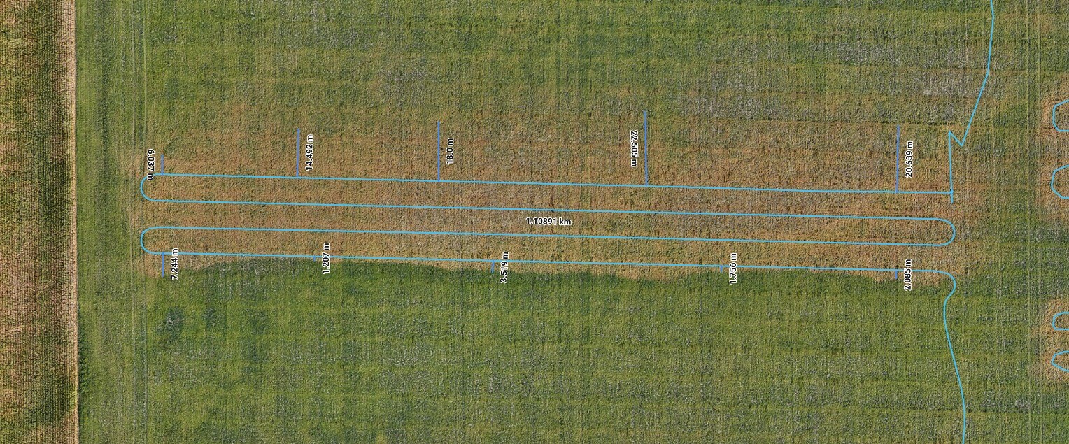
    The second method overlays the flight path onto the area burned. The upwind side of the swath was determined from an average of at least five measurements along the upwind flight path. The downwind side of the swath was calculated the same way (Figure 5). Both the average upwind and downwind distances were added to arrive at the ESW. Hereafter referred to as the “port + starboard extent” method. This approach captures a clear representation of the upwind side of a single pass, but overestimates ESW by including any cumulative increase in drift from multiple passes on the downwind side.

    Figure 5 – Example of port and starboard measurements along the downwind and upwind-most flight paths. The averages were calculated and added to estimate effective swath width.

    Results – Part One

    Planned versus Measured Treatment Area

    The “programmed swath width” is something of a misnomer. More accurately, it is the route spacing and it describes the distance between passes over a target area. However, most drone manufacturers refer to this variable as programmed swath width, so that’s what we’ll do.

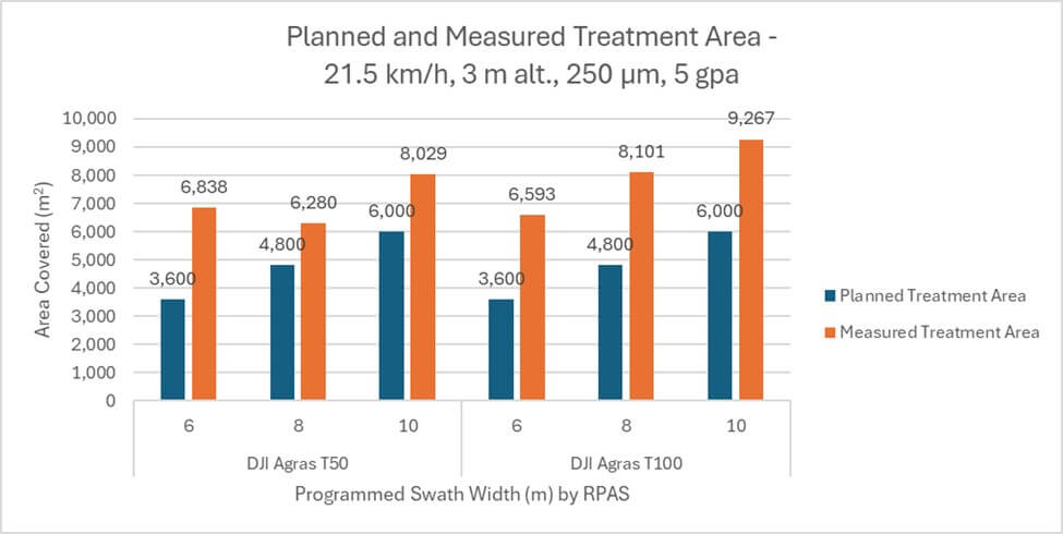
    Planned treatment areas were calculated from distance flown × programmed swath width × number of passes. Measured treatment areas were calculated by tracing a polygon along the perimeter of the area burned. In all cases, actual was larger than planned by an average 36.1%. The T50 treated 32% more area than planned and the T100 treated 40% more area than planned, or 8% more than the T50 (Figure 6).

    Figure 6 – Planned and Measured Swath Widths for T50 and T100.

    Programmed and Effective Swath Widths

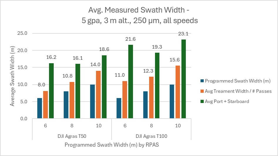
    In all cases, the “treatment width ÷ passes” method produced an estimated ESW that was greater than, and positively correlated with, programmed swath width (Figure 7). For the T50, it was an average 26.8% wider. For the T100, it was an average 38.3% wider. The ESW calculated by the “port + starboard extent” method was larger still, but was not positively correlated with programmed swath width. For the T50, it was an average 52.8% wider. For the T100, it was an average 62.5% wider.

    No matter the method used to estimate ESW, the T100 exceeded the planned swath width by more than the T50. Using the “port + starboard extent” method, the average T100 ESW was 21.3 m, which is an average 15.4% wider than the average 17 m ESW produced by the T50.

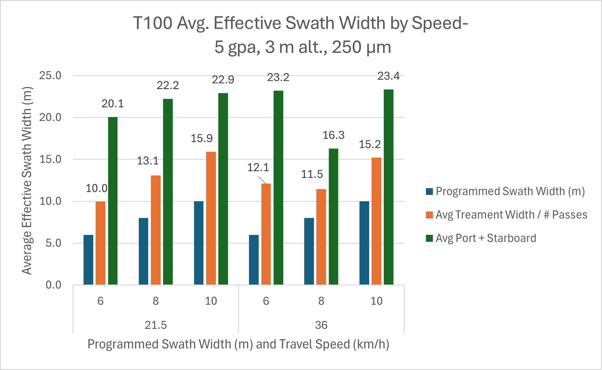
    Figure 7 – Average measured swath width (two methods) compared to planned swath width for the T50 and T100 flown at 5 gpa, 3 m altitude, 250 µm spray quality and multiple speeds.

    T50 ESW by Travel Speed

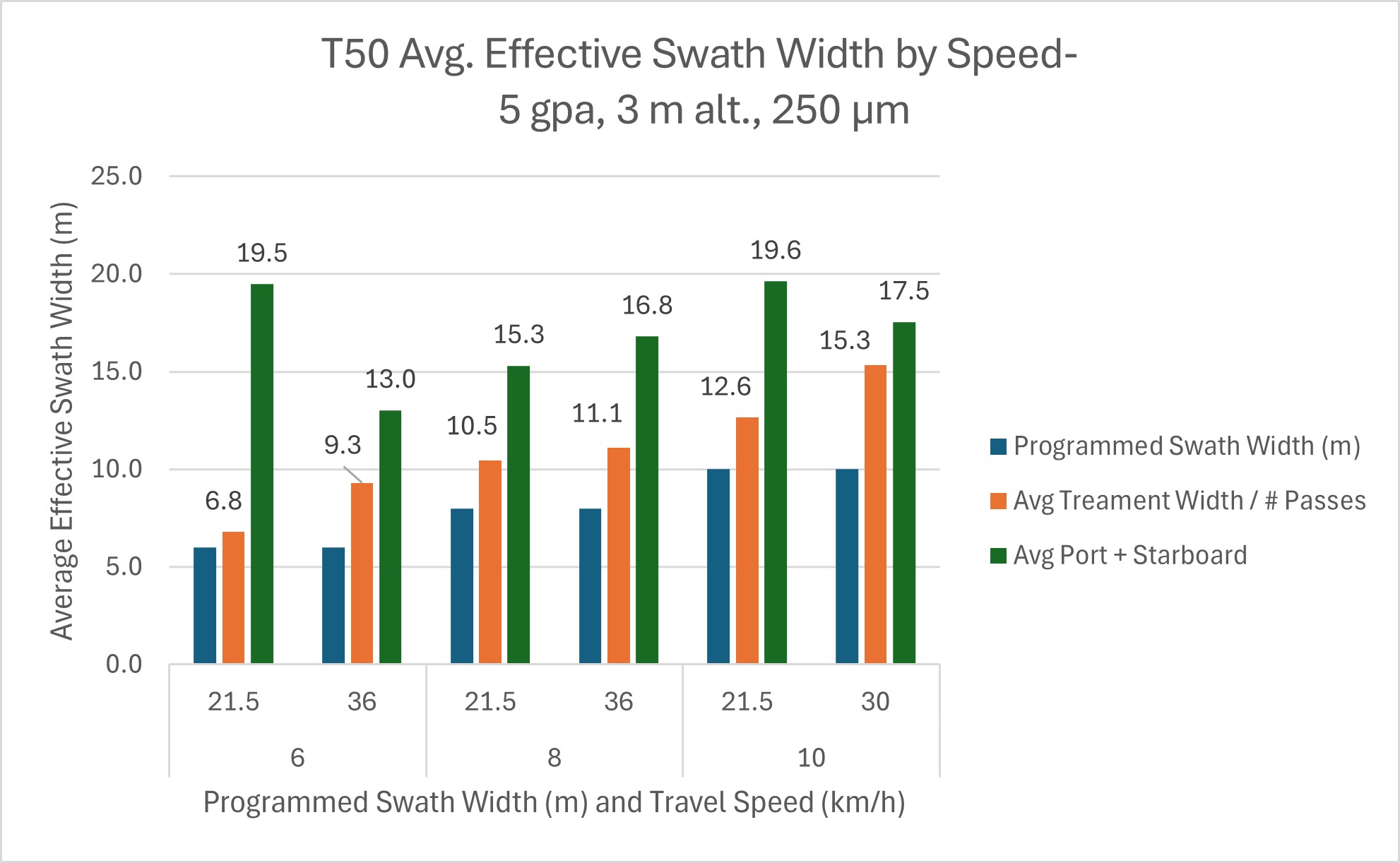
    When travel speed becomes the independent variable for the T50, the “treatment width ÷ passes” method produces an average ESW that positively correlates with flight speed. At 21.5 km/h, the average ESW was 10 m, increasing to 11.9 at 30-36 km/h (Figure 8). This is typical and expected as higher speeds have been shown to produce wider swaths with the T10 and T50.

    However, the relationship between speed and ESW is less clear when estimated using the “port + starboard extent” method. At 21.5 km/h the average swath was 18.2 m, but reduced to 15.8 km/h at 30-36 km/h (Figure 8).

    Figure 8 – Average measured swath width by speed for the T50.

    T100 ESW by Travel Speed

    When travel speed becomes the independent variable for the T100, neither method for estimating ESW show an effect from flight speed. The “treatment width ÷ passes” method produced an average ESW of 13 m at 21.5 km/h and 12.9 at 30-36 km/h (Figure 9). The “port + starboard extent” method produced an average ESW of 21.7 m at 21.5 km/h and 21 at 30-36 km/h.

    Figure 9 – Average measured swath width by speed for the T100.

    Results – Part Two

    T100 ESW by Travel Speed

    The effect of flight speed on treated area and ESW was examined. In each case, the treated area was significantly larger than the programmed area (Figure 10).

    Figure 10 – Actual treatment areas compared to expected for the T100; three speeds.
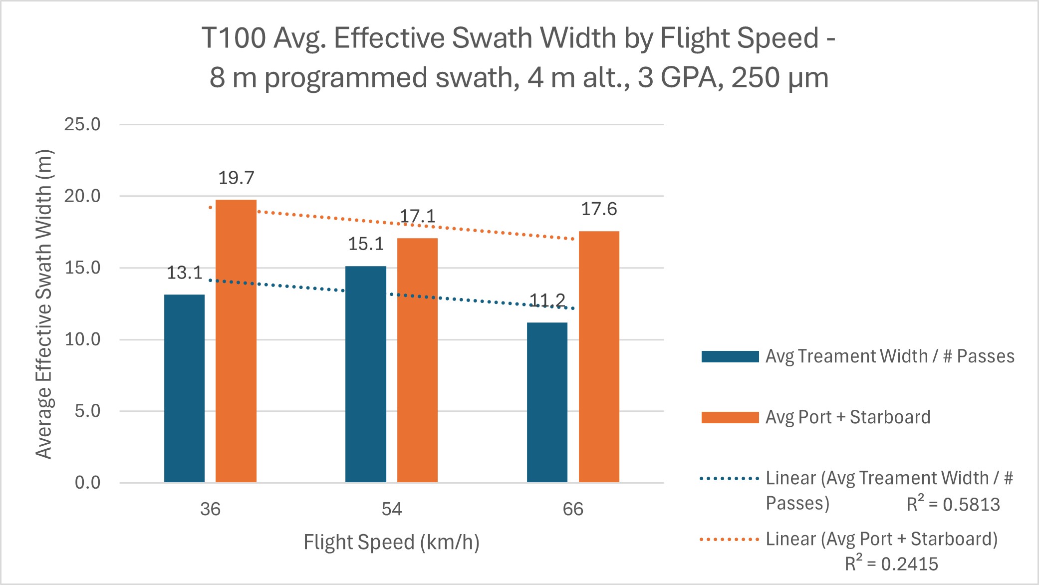
    Similar to Part one, travel speed did not appear to influence ESW in any consistent or significant way (Figure 11).

    Figure 11 – Average swath width for T100 calculated using two methods at three speeds.

    T100 ESW by Spray Quality

    The effect of spray quality on treated area and ESW was examined. Once again, in each case, the treated area was significantly larger than the programmed area (Figure 12).

    Figure 12 – Actual treatment areas compared to expected for the T100 using three spray qualities.

    Effective swath widths estimated from both methods were negatively correlated with spray quality (Figure 13). Coarser droplets have greater mass, making them are less prone to displacement by wind than finer droplets. The “treatment width ÷ passes” saw an 80 µm spray quality produce an ESW 46.8% larger than a 500 µm spray quality. The “port + starboard extent” method saw an 80 µm spray quality produce an ESW 22.6% larger than a 500 µm spray quality.

    Figure 13 – Average swath width for T100 calculated using two methods for three spray qualities.

    Discussion

    In all cases, the area treated (i.e. burned) exceeded the area planned. The T50 covered 32% more area while the T100 (with the same operational use case) covered 40% more. This implies that the T100 created wider swaths and/or drifted more than the T50.

    The ESW estimated from herbicide efficacy appears to be considerably larger than those observed in fungicide efficacy / coverage studies. This is likely the result of the agronomic use case. Consider that herbicides have a relatively lower threshold dose than fungicides. Further, herbicide application on bare earth or into sparse canopies permits the lateral spread of droplets, where spraying fungicides into a dense canopy limits penetration in all directions. Even the sparsest coverage from a systemic herbicide (especially when used at the highest label rate, as done here) produces a visual effect, and this binary result (i.e. hit or miss) likely exaggerates the effective swath width. Nevertheless, this should raise awareness of the importance of field boundaries and margins, particularly with herbicides.

    When estimating ESW, the method used affected the results. The “port + starboard extent” method resulted in large and low-resolution estimations of ESW, whereas the “treatment width ÷ passes” method seemed to respond in a more predictable way, even if it underestimates the ESW. Ultimately, both methods produce rough estimates that are likley exaggerated becuase of the high dose; they are not intended to replace traditional, quantifiable assessment methods.

    With that caveat reaffirmed, we assessed ESW using the “treatment width ÷ passes”. It was positively correlated with flight speed for the T50, as observed in previous work. However, this was not the case with the T100. Given that both drones were operated using the same settings, it is unclear why the T100 would produce such erratic results. Future work will evaluate T100 ESW using conventional methods.

    When the T100 was flown using a span of three droplet sizes, there was a strong negative correlation between average droplet size and ESW. Once again, this aligned with previous experience. While rotary atomizers on drones tend to create smaller droplet sizes than reported by the flight controller, coarser droplets have greater mass, making them less prone to displacement by wind.

    However, when the T100 was flown at at three speeds, the relationship with ESW was once again unclear. When flown at 36 km/h (~10 m/s) the T100 was flying at the top speed of the T50. It also flew at 54 km/h and at 66 km/h, which was the highest speed we could achieve at 5 gpa. The ESW (as estimated using the “treatment width ÷ passes” method) was essentially unchanged. While it is possible (and likely) that any increase in effective swath width due to travel speed was obscured by drift, previous work has shown that drift increases concomitantly with speed. There was no burn pattern to indicate drift, here.

    Perhaps this is a function of a greatly reduced dwell time diminishing the effect of the downwash. Or, perhaps, the T100’s capacity for higher speeds has allowed it to pass beyond translational lift into true forward flight, similar to a helicopter. Translational lift occurs any time there is relative airflow over the rotor disk. As headwind and/or forward speed increase, translational lift increases, resulting in less power required to hover. According to Transport Canada, it is present with any horizontal flow of air across the rotor but most noticeable when the airspeed reaches 16 to 24 knots flight (8.25 to 12.8 m/s or 30 km/h to 46 km/h). This would greatly reduce the effect of the downwash on droplet movement. In our first impressions of the T100, we found that flying slower overheated the battery. This did not occur at higher speeds, and this efficiency supports the premise that it moved past translational lift, perhaps achieving true forward flight.

    If this theory is correct, it’s a new development for rotary drones, which were not previously capable of reaching these speeds. Downwash was an unavoidable side effect of the flight, but may now be a tool for the operator to use as the situation warrants – battery temperature notwithstanding. Perhaps it warrants a return to horizontal booms positioned beyond the downwash in order to improve coverage uniformity. On the other hand, we saw that it took the T100 roughly 100 m to reach the target 66 km/h, meaning it moved from hover to translational flight and beyond over that distance. This raises questions about how the spray would respond throughout that transition.

    More work is required.

    Acknowledgements

    Adrian Rivard and Stuart Hunter (Drone Spray Canada), Adam Pfeffer (Bayer Canada) and Mike Cowbrough (Ontario Ministry of Agriculture, Food and Agribusiness) are gratefully acknowledged for their participation, and both in kind and financial support of this study. Thanks also to Mark Ledebuhr and Tom Wolf for discussions surrounding the interpretation of these results.