Author: Jason Deveau

  • Methods for Applying Fungicides in Corn

    Methods for Applying Fungicides in Corn

    This work was performed with Albert Tenuta (OMAFRA) and David C. Hooker (University of Guelph, Ridgetown).

    Objective

    Gibberella ear rot is a significant disease that reduces the quality of grain corn, especially with the accumulation of mycotoxins (such as Deoxynivalenol (DON)) produced from the causal pathogen(s). Infection occurs through the corn silk channel when ideal temperatures (~27°C) and high humidity are present. Cool, wet conditions after pollination favour disease development and determine the degree of infection. With crop management practices providing only modest improvements in disease control, strategies to increase the efficacy of fungicides are important to investigate. Research has shown that the timely application of fungicide labelled to suppress the disease can reduce mycotoxins, but only by ~50%. We wondered if changes in the method of application could give better results.
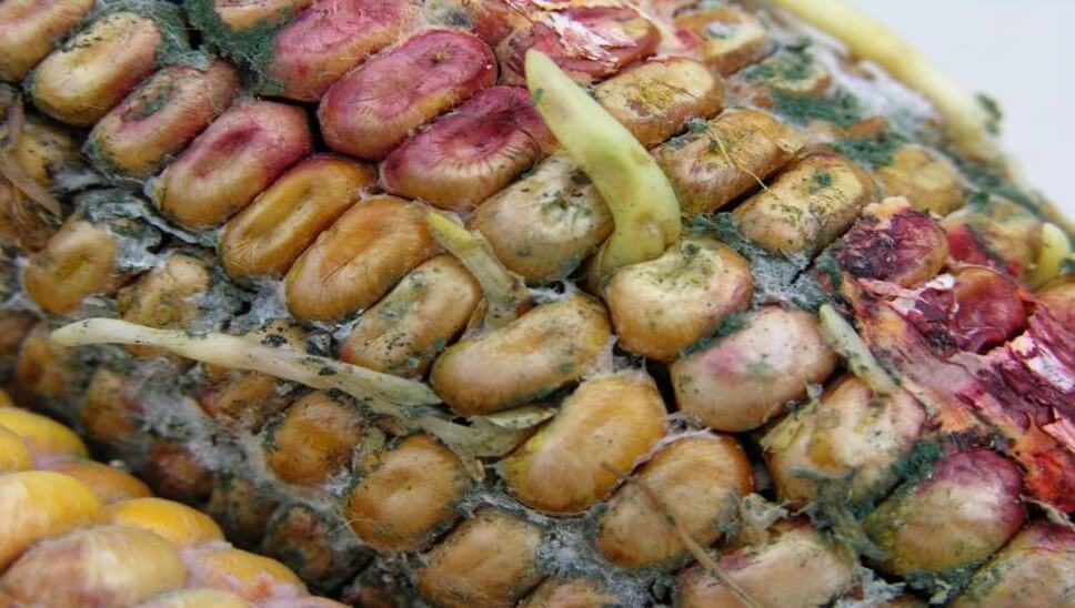
    Gibberella ear rot

    It is reasonable to assume that improvements in spray deposit uniformity and increases in overall spray coverage (up to some threshold) at the infection channel (i.e. the silks) should result in improved efficacy. Water sensitive paper is an excellent tool for the qualitative evaluation of spray coverage. However, recognizing the complicated relationship between dose and coverage, we also looked at the deposition of copper sulphate as a surrogate for active ingredient .

    Our primary objective of this study was to compare various sprayer systems and nozzle configurations by evaluating both spray coverage and copper sulfate deposition at the silks.

    Experimental Design

    The test field of hybrid corn had a stand of ~80,000 plants/ha. It was located at Ontario’s U of G Ridgetown Campus and was managed similar to a grower’s field (e.g. fertility, etc.). In August of 2019 we evaluated nine sprayer rigs (or nozzle configurations) in a randomized block design.

    The ground rigs were calibrated to deliver a spray volume of 190 L/ha and the aerial systems to deliver 47 L/ha.  In order to achieve the target spray volume, the ground rig speed varied from 9.5 to 13 km/h, depending on nozzle configuration. The aerial applicators used the same nozzle configuration, travel speed and altitude as in their commercial field applications.

    SprayerNozzle SetNotes
    John DeereYield Center 360 UNDERCOVER drop pipes 75 cm (30″) spacing, each equipped with two Turbo TeeJet (TT) nozzles.Drop pipes were centred between corn rows with nozzles adjusted to spray ~horizontally and directly at the corn silks.
    John DeerePentair Hypro Guardian Air nozzles on 50 cm (20″) spacing.Boom positioned to create 100% spray overlap at tassel height.
    John DeereTurbo TeeJet Induction (TTI) nozzles on 50 cm (20″) spacing.Boom positioned to create 100% spray overlap at tassel height.
    John DeereTurbo TeeJet (TT) nozzles on 50 cm (20″) spacing.Boom positioned to create 100% spray overlap at tassel height.
    New Holland (front-mounted boom)Wilger 60 degree conventional flat fan nozzles on 40 cm (16″) spacing.Boom positioned to create 100% spray overlap at tassel height.
    New Holland (front-mounted boom)Wilger 60 degree conventional flat fan nozzles alternating with custom-made Wilger 40 degree conventional flat fan nozzles on 40 cm (16″) spacing.40 degree nozzles were positioned between corn rows (interrow) while 60 degree nozzles were positioned over the tassels.
    Hagie (front-mounted boom)Drop hoses terminating with TeeJet Duo Nozzle bodies equipped with Turbo TeeJet Induction (TTI) nozzles were alternated with TeeJet XR110 nozzles.Drop hoses were centred between corn rows but nozzles were not aimed directly at the corn silks (aimed down 45 degrees and spray parallel to ground rather than perpendicular). They alternated with the AI nozzles positioned over the tassels.
    HelicopterAir Induction TeeJet Turbo TwinJet (AITTJ) nozzles directed backwards.
    AirplaneCP-111T nozzle bodies with CP256-4015 40 degree flat fan tips on 15 cm (6″) spacing.Wingspan was 14.2 m with a 10.6 m boom width.

    The field was divided into four replicated blocks (REP 1-4 in the image below) which corresponded with a single pass of the sprayer. The sprayers alternated direction with each pass over the four blocks. Depending on the ground rig, a single pass through a block might include more than one set of nozzles. For example, in the image below, a John Deere sprayer carried a different nozzle set on each of four sections, leaving the centre boom section off. Therefore, each block was subdivided into four experimental units that corresponded with each nozzle set. Further, to account for variability, each experimental unit was further subdivided into five ranges. Four water sensitive papers (yellow rectangles) were oriented sensitive-side up and fastened to random corn plants directly on top of silks at each of the five intersections between range and treatment for a total 20 papers. This was replicated four times for a final count of 80 papers per treatment.

    The experimental unit covered by a nozzle set was four corn rows wide (~3 metres). Space was left between each boom section to provide a buffer and no nozzles were placed on the centre boom section. Four water sensitive papers (yellow rectangles) were fastened to random corn plants directly on top of silks at the intersection of each range and for a total 20 x 4 = 80 papers. The chevrons indicate sprayer direction.
    Test plots at University of Guelph, Ridgetown Campus

    Evaluating Coverage

    Each sprayer applied copper sulphate (Plant Products Inc., Leamington, ON) at 2 kg/ha as a chemical tracer. Agral 90 was added to the spray solution at 0.1% (v/v) to better emulate a typical fungicide application. After spraying, each water sensitive paper was allowed to dry, collected and then digitized using a DropScope (SprayX, Sao Carlos, Brazil). Droplet density and percent surface covered were evaluated within the detection limits of the equipment. Dose (represented by deposit volume) was more relevant to this study than percent surface covered, so a spread factor was used to convert area covered to volume. Once the papers were scanned they were subjected to flame emission spectroscopy (FES) (Actlabs – Activation Laboratories Ltd., Ancaster, ON) to determine the amount of copper deposited.

    DropScope digitizing water sensitive paper

    Results

    Deposit area and volume

    Note that papers were placed singly, oriented face-up. This was a missed opportunity to explore abaxial (down-facing) coverage and may have created a small experimental error wherein deposition from copper sulphate would be accounted for on both sides, but would only resolve on one side for area and density analysis. The results from evaluating water sensitive paper suggest trends and serve as quality checks for the experiment.

    The percent area covered on water sensitive papers was affected by nozzle configuration (P<0.0001). Ground rigs produced ~4.0-12.0% area coverage, while aerial produced ~0.7-1.0%. It is not appropriate to compare ground and aerial spraying using water sensitive paper. Water sensitive paper does not reliably resolve deposits under ~60 µm and therefore underestimates the deposits from aerial applications because their spray quality tends to be finer. Further, these figures have not been normalized to reflect the differences in sprayer volume (190 L/ha for ground versus 47 L/ha for aerial).

    The nozzle configurations with the highest percent area covered were produced by the 360 Undercover drop pipes and the TeeJet drop hoses (~9.5-12.0%). Coverage variability increased with percent area covered, but the lower 95% confidence limit with the pipes and hoses still exceed the upper limit of all overhead broadcast nozzles.

    Yield Center 360 UNDERCOVER drop pipes

    When area covered was converted to volume, estimated deposit volume on water sensitive papers was also affected by nozzle configuration (P<0.0001). The estimated volume calculated from deposit area showed fewer statistical differences across nozzle configurations compared to area data. However, once converted, there was no statistically significant difference in the volume deposited by drops or most broadcast methods.

    Copper deposition

    FES residue analysis (i.e. evaluating the amount of copper deposited on targets expressed as mass density) complements the water sensitive paper data. There are some differences that should be noted:

    • All applications sprayed the same amount of tracer per planted area. As such, depositions are more fairly compared with no need for normalization.
    • FES can resolve copper deposits as low as 0.5 µg/sample and may be more sensitive than the WSP method, which does not reliably resolve deposits under ~60 µm.
    • WSP will only resolve coverage on one surface. However, when these papers are subjected to FES, deposits on both sides of the paper will be accounted for, providing a more accurate result.

    As anticipated, there was no correlation between the area coverage or volume estimates and the FES-derived copper deposition data. Estimated copper mass density on water sensitive papers was affected by nozzle configuration (P<0.0001). Analysis showed 56% more copper deposited from the 360 Undercover nozzles (1.75 µg/cm2) compared to the next highest deposition (1.12 µg/cm2) which was from the drop hose configuration (P<0.05). We feel the TeeJet drop hose configuration would have performed better still had the nozzles been directed at the silks, and the alternating broadcast nozzles been omitted and flow redistributed to the nozzles on the drops (see below).

    Copper deposition from the airplane was similar to ground rigs with broadcast overhead nozzle configurations. The airplane deposited ~2x the copper as did the helicopter. It is assumed this is because the rotary atomizer nozzles on the airplane produced a much finer spray quality than the TTI nozzles on the helicopter. This increased the number of droplets considerably and has been shown to produce better coverage, particularly at such low sprayer volumes. Learn more about droplet size and behaviour here.

    Average copper deposition from the Guardian Air nozzle set was similar to all other ground sprayer overhead broadcast setups, but had the highest variability (Between 0.4 and 1.12 µg/cm2). Comparatively, the lower 95% limit of the 360 Undercover drop pipe deposited 3.4x the copper as the lower limit of the Guardian Air.

    Conclusions

    • The best deposition was produced from the Yield Center 360 Undercover drop pipes, followed closely by the TeeJet Duo nozzle body on drop hoses.
    • The deposition from ground sprayers with overhead broadcast nozzles was ~30% less than that of the two drop nozzle systems tested.
    • The deposition from Guardian Air and TTI nozzles were among the lowest of broadcast nozzle configurations with higher variability, but differences tended not to be statistically different (P=0.05) compared to other broadcast nozzles.
    • The deposition from the airplane was similar to the ground rig overhead broadcast applications, but the helicopter deposited the lowest amount of copper overall, likely due to droplet size (see image below).
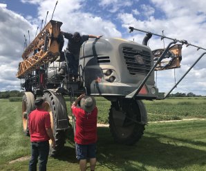
    Helicopter with air induction TeeJet Turbo TwinJet (AITTJ) nozzles directed backwards.

    Next steps

    In the summer of 2022 we re-evaluated promising nozzle configurations from this study, as well as other application methods (see bulleted list below).

    • Include various RPAAS (remote piloted aerial application systems) designs.
    • Include the Agrotop Beluga drop hose (Greenleaf Technologies, Louisiana, USA) with two nozzle bodies to span the silking zone of the canopy.

    We used water sensitive paper as a qualitative indicator, but folded them to get adaxial and abaxial data. We also used copper deposition to indicate dose. Once the results are analyzed we’ll write a companion article to this one.

    In 2021 and 2022 a separate study was performed to evaluate the efficacy, ease-of-use and return on investment of the Beluga drop hoses in corn. An article describing that work can be found here.

    Thanks to the agrichemical companies, students, equipment owners and operators that donated their time and equipment to make this study possible.

    Bonus

    Watch these very cool slow-motion videos of the airplane and helicopter applications. Note that there is no difference in how the spray behaves once released; It deposits as a function of wind, gravity and momentum and is not “blown in” by the helicopter.
  • Venting Liquid-Filled Pressure Gauges

    Venting Liquid-Filled Pressure Gauges

    Liquid-Filled or Dry?

    Small-plot agricultural sprayers should have a pressure gauge on the wand or boom to ensure accurate application rates. Most are added after-market and the operator has the choice of buying liquid-filled or dry gauges.

    Glycerine- or silicone-filled gauges are preferred because they dampen pressure spikes, pulsation and mechanical vibration. Compared to dry gauges, they are available in higher ranges and are less prone to moisture problems (which cause corrosion, accuracy and visibility issues).

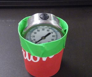
    We use 100 psi (~7 bar) liquid-filled gauges for our handheld sprayers. Only recently did we acknowledge the sticker affixed to the glass advising the user to cut the nipple off the rubber plug located at the top. Preferring to avoid messy leaks, we have always left it intact.

    We wondered what impact, if any, this was having…

    What are Vents?

    Expensive gauges have mechanical vents that can be opened prior to use and closed to retain liquid when stored. More commonly, there is a rubber plug with a protrusion (referred to as a nipple).

    Why Vent?

    Mechanical, liquid-filled gauges are sealed to keep the liquid in. When there are temperature fluctuations, the liquid expands or contracts and creates “case pressure”. This exerts a force that interferes with the pressure reading.

    According to Marshall Instruments, case pressure can offset the accuracy by approximately 1 psi (0.07 bar) for every 35˚F (20˚C) temperature change, but is only noticeable when measuring lower pressures (0-15 psi or 0-1 bar). Nevertheless, they advise all gauges should be vented prior to use.

    The plug can be removed to allow the user to refill the gauge, maintaining an air space of about ½” at the top of the window. If the nipple is cut off, the gauge is permanently vented and will leak if the gauge is not kept vertical.

    Testing

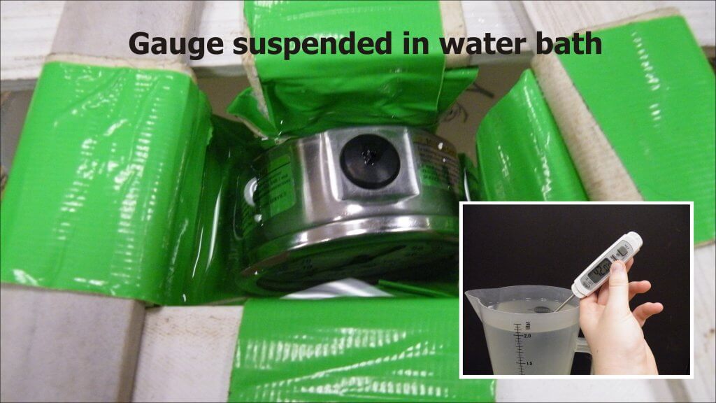
    We performed an experiment to see if typical working temperatures had a practical impact on the accuracy of an unvented gauge. We suspended an unvented, liquid-filled gauge upright in a water bath at approximately 15˚C, 30˚C or 45˚C (59˚F, 83˚F or 113˚F) until it equilibrated. The high temperature may seem unreasonable, but gauges left in trucks on summer days get far hotter.

    The gauge was quickly removed and placed in a manometer (Ametek T-975) where it was subjected to pressures of 15, 30 and 45 psi (1 bar, 2 bar and 3.1 bar) and readings recorded. This was repeated five times. We then vented the gauge and repeated the process.

    Results

    At first, there appeared to be very little difference in average accuracy of vented and unvented gauges. Accuracy refers to the closeness of a measured value to a standard or known value. Perhaps there was some small increase in the pressure reported by an unvented gauge, but very little practical difference.

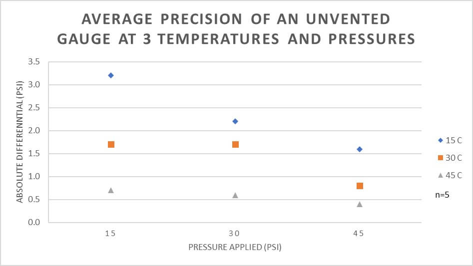
    However, when we look at variability we get a different picture. Variability is a measure of precision, which refers to the closeness of measurements to one another. The graphs show that an unvented gauge has greater variability (less precision) at lower temperatures and lower pressures.

    A good way to think of accuracy and precision is using the classic archery bulls-eye metaphor. The unvented pressure gauge is best represented by the third image, where it is accurate (on average) but not precise (variable).

    Real-World Example

    What does this mean in practice? Consider someone spraying a small plot using a TeeJet XR8002 nozzle on a CO2-powered hand boom at 30 psi. The difference in output between 30 psi and 40 psi is about 0.003 gpm / psi.

    An unvented pressure gauge used on a hot day may read 1.5 psi lower, causing you to overcompensate and raise the pressure 1.5 psi higher than intended. That would result in 0.0045 gpm (0.5%) more applied. Compensating for an unvented gauge on a colder day might be closer to 0.009 gpm (1%) more applied.

    Assuming a walking speed of 3.1 mph (5 km/h) and a swath of 20” (50 cm), the nozzle should emit about16.3 gpa at 30 psi. Unvented in the heat, that’s 16.7 gpa. At 33 psi, that’s 17.15 gpa. That’s almost 1 gpa more than intended. Potentially, the lack of precision could make a significant difference.

    Conclusion

    • Liquid-filled gauges are preferred over dry gauges.
    • To ensure precision, the gauge should be vented prior to use.
    • Permanent venting on a hand-held sprayer causes leaks, which is a nuisance, so we suggest simply lifting the edge of the plug with a screwdriver or fingernail to vent the gauge prior to each use.

    This work was performed by OMAFRA summer student, Aidan Morgan.

  • Paint it black – Parody

    Paint it black – Parody

    Never fail, as spring turns to summer we get questions about algal growth in water tanks. There are lots of suggested solutions, but questions about pH antagonism and phytotoxicity seem to linger. In 2021/22 we ran trials to explore how well home-grown algicides like copper, bleach, and ammonia work, and whether they cause antagonistic responses when that carrier water is used on crops. You can see the results here.

    Anticipating those results, we wrote this parody on a Stone’s classic. Not long after it was brought to life by the brilliant minds behind Michigan’s epic podcast “The Vegetable Beet” (Go subscribe right now!). You can hear it in the link below, where Ben Phillips is accompanied by his daughter’s toy tambourine. Crank it up to 11!

    You can even download Ben’s sheet music here.

    I see a white tank and I want it painted black
    No algae anymore, I want my water back
    I see the cart drive up while spraying summer rows
    I have to dump it out until the algae goes

    I see my neighbours’ tanks and they’re all painted black
    With copper sulfate they claim algae won’t come back
    I see them turn their heads and quickly look away
    They see my algae grow in sunlight every day

    I look inside the tank to see if it is black
    I could park it in the shed, or in the shade out back
    Maybe then it’ll fade away and I can face the facts
    It’s not easy filling up when your filters plug with crap

    I wish that my green sea would turn a deeper blue
    If you try chlorine pucks it will clear up for you

    I’ll store my tanks away from that bright summer sun
    Then I’ll spray algae-free before the mornin’ comes

    I see a clean tank ‘cause I had it painted black
    No algae anymore, I got my water back

    I see the cart drive up while spraying summer rows
    Clear water coming out, and no more clogging woes

    Hmm, hmm, hmm
    Hmm, hmm, hmm
    Hmm, hmm, hmm
    Hmm, hmm, hmm

    I want to see your tank painted black!
    Black as night!
    Black as coal!
    I wanna see the bugs, knocked right out of the sky
    I wanna see it painted, painted, painted black, yea!

  • Oh the Places You’ll Spray – Parody

    Oh the Places You’ll Spray – Parody

    Enjoy our take on a Dr. Seuss work-of-art. We’re sure the fine doctor would want to end resistant pig weed’s reign of terror as much as we do. Hear us recite it in the sound bar, read it yourself, or head to the bottom of the article to see the talented Bridgette Readel (@bmreadel) read it for you. Enjoy!

    Press Play to hear the audio version of this article

    In the home farm’s west field,
    where the soybeans won’t grow,
    and the wind blows the soil from deep tillage you know,
    and no pollinators come, excepting old crows
    is the patch of resistant pigweed.

    And downhill in the boundary, some neighbours say,
    if you look close enough you can still see today,
    where herbicide persisted,
    in the places it drifted,
    from the winds that took it away.

    How did it drift?
    How did it get there?
    And why was it lifted and taken somewhere
    from the home farm’s west field where the soybeans won’t grow?
    Look to the sprayer.
    Look close, and you’ll know.

    You won’t see Coarse nozzles.
    You will see high booms
    that wobble and bounce on a sprayer that zooms
    in headwinds too high
    in the late afternoon.
    They may even spray by the light of the moon!

    Check the chemical shed.
    Crack the door, just a fraction.
    You’re likely to see
    A lone mode of action.

    “Tell me how,” says the farmer
    “I’ll do what you say.”
    “But I only have so many hours in the day
    to spray the west field where the soybeans won’t grow,
    and battle the pigweed that simply won’t go.”

    “Oh the things you can do! So much can be done!”
    “Learn to spray in light winds, in the day, in the sun!”
    “Lower booms, use more water, use droplets so Coarse.”
    “We’ve told you before…
    (you will note we are hoarse.)”

    The farmer said nothing, just gave us a glance.
    We could tell he was thinking of time, effort and cash.
    “Driving slow improves coverage,
    and you can make up the time,
    with faster fills, longer booms, and more precise A-B lines.”

    That was long, long ago.
    Let’s check in today,
    and see if the problems have withered away.

    In the home farm’s west field,
    where the soybeans now grow,
    and cover crops cling to the soil down below,
    the pollinators buzz because drift doesn’t blow.

  • Crop-Adapted Spraying (CAS) and an Apple Orchard Case Study

    Crop-Adapted Spraying (CAS) and an Apple Orchard Case Study

    An orchard spraying scenario

    Here’s a common situation: An orchardist following IPM identifies a pest that poses an economic threat. It’s an annual pest and spraying is really a matter of when, not if. The operation is 150 acres and runs three airblast sprayers; two have a tower and one does not. Multiple varieties are planted in several blocks on different rootstocks and they are at different stages of maturity. The newer blocks are trellised high density trees and the older blocks are semi-dwarfs on different row spacing. Let’s also imagine the pruning team hasn’t finished yet, so some trees are not pruned.

    The orchardist turns to the pesticide label to decide how to spray such variable targets. It prescribes a range of doses per planted area (not canopy size), depending on the pest pressure. It advises the orchardist to use “enough water” to ensure “good coverage” without incurring “runoff”.

    The orchardist recognizes that the label is vague, and elects to rely on what has worked historically: A water-soluble pouch is dropped into each tank (dose is close enough), and each sprayer operator is instructed to drive at an efficient speed (get it done because rain is coming), spraying until the tank is empty. They say that if a tank is running low before the job is done, speed up and stretch it. If the spray is overshooting a younger planting, they suggest turning off the top nozzles and/or driving faster.

    Airblast operators face this situation regularly. The question is: “Is there a problem with spraying this way if it results in a respectable crop of quality fruit?” Agricultural engineers specializing in application technology in Spain, Australia, Great Britain and the United States say there is a problem, and on behalf of Canada, I completely agree with them.

    Canopy and Sprayer Variability

    The fundamental problem is inconsistent spray coverage and avoidable waste (of time, water and pesticide) due to variability. Our scenario notes multiple sprayer operators, different models of sprayer, and a range of varieties, orchard architectures and canopy management practices. The label does not allow for any of these factors, adhering to a rate based on planted area and remaining silent on water volume.

    International peer-reviewed journal articles stretching back to the sixties have conclusively demonstrated order-of-magnitude differences in the area-density of orchard canopies from one acre to the next. There can even be fold-differences in canopy area-density in the same planting as the season progresses. A label prescribing a fixed dose based on the area planted is not appropriate for any vine, bush, cane or tree crop, and the result is that more crops are over- or under-sprayed than receive appropriate coverage.

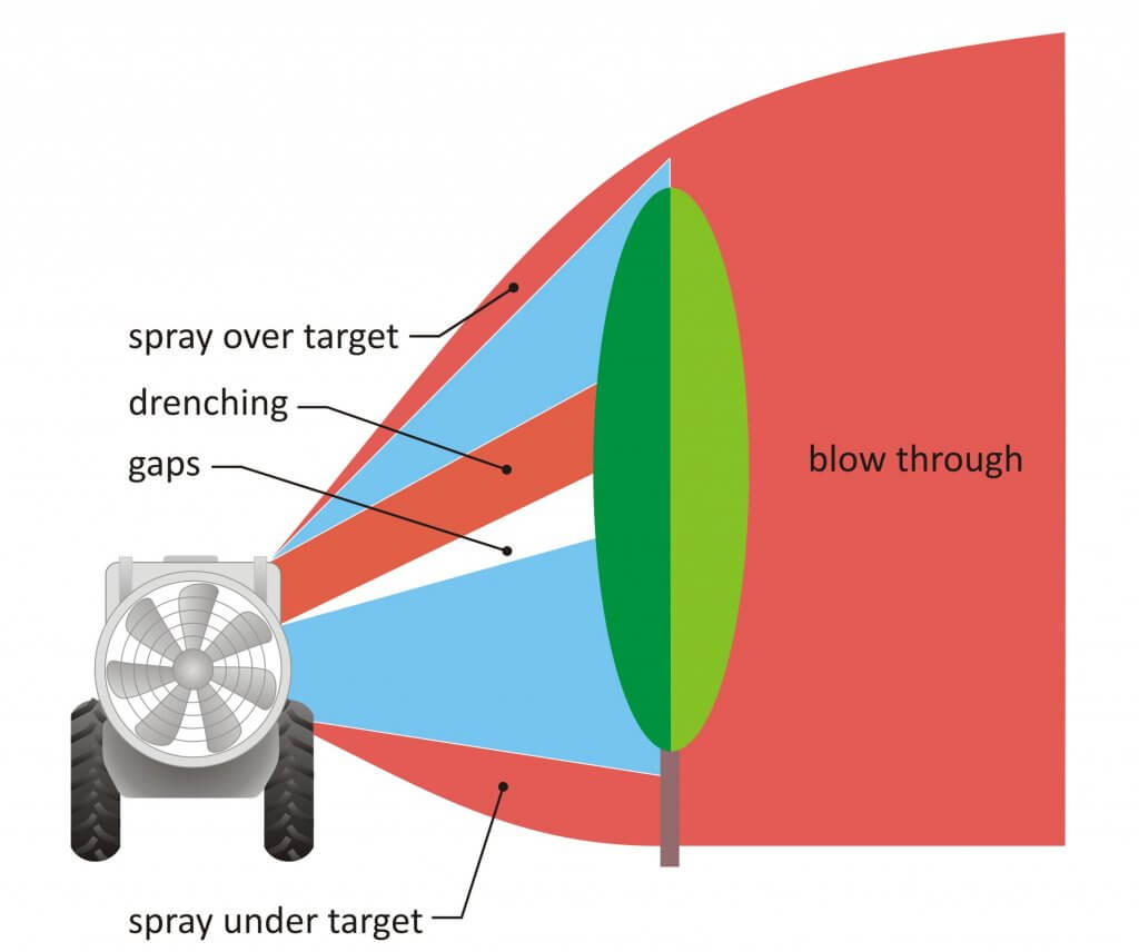
    Let us not forget the variability that comes from a poorly adjusted sprayer. I won’t to attempt to quantify the impact (although some researchers have suggested order-of-magnitude differences from sprayer to sprayer). Instead, let’s illustrate it as a conceptual “before and after”:

    Before: Potential spray loss and inconsistency before adjusting sprayer to match the canopy
    After: Coverage variability reduced and unnecessary waste mostly eliminated.

    Beyond the immediate impact on efficiency, variability makes it difficult to diagnose pesticide effectiveness. As an example, there was a scab outbreak in Ontario in 2009 that elicited questions about timing, weather, product choice and resistance. There was very little attention given to spray coverage, which to my mind should have been the first question if only to eliminate it as a potential culprit. This is because each operation interprets labels differently, and very few confirm coverage in any quantifiable way. This practice makes it more difficult to identify a cause when crop protection fails.

    Optimizing pesticide rates

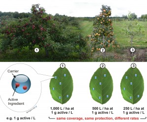
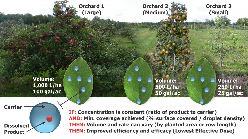
    That was a lot of preamble to describe an issue that many orchardists are already aware of. What is needed is a way to adjust the amount of pesticide per unit ground area (i.e. the label’s prescription) to achieve consistent foliar coverage for canopies of varying shape and density. The concept is visualized in the following figure. In addition, the method has to be simple, intuitive and effective.

    Many models have been proposed to tackle the dose expression issue, including Tree-Row Volume, Leaf Area Index, Leaf Wall Area, PACE+ and DOSAVIÑA. There are advantages and disadvantages to each method. Standing on the shoulders of giants, we combined aspects of each of these models, including incorporating coverage factor research from USDA ARS work in nurseries, to develop the Crop-Adapted Spraying (CAS) method. It is neither complicated nor sophisticated. It formalizes a series of qualitative calibration techniques and the objective is to achieve a target foliar coverage pattern. When achieved with sufficient accuracy, pesticide efficacy is maintained and waste is greatly reduced.

    Caveats

    Perhaps I shouldn’t point out flaws before I describe the model’s effectiveness, but it’s important to understand that CAS relies on a few critical assumptions.

    The first assumption is that the sprayer operator’s typical ratio of formulated product to carrier is appropriate. We need a starting point for adjusting the amount of pesticide per unit planted area, and unless the label specifies a concentration (i.e. a ratio of formulated product to water) or a minimum amount of product per planted area, this is a reasonable starting point. The appropriateness of this assumption is evidenced by a history of satisfactory pest control in the orchard.

    The second assumption lies in defining a threshold for sufficient coverage, and this is a real challenge. Applications can be concentrate or dilute. Some products translocate in the leaf or redistribute on the leaf surface while others do not. Even the droplet size employed (e.g. A mist blower’s fines compared to Medium-Coarse droplets produced by an air induction nozzle) will affect dose, bioavailability and how long residues are active. So, how does one draw a universal line in the sand and say “this much is enough”?

    Our threshold for suitable foliar coverage has evolved through experience, literature review and independent experimentation in several countries and in multiple 3D cropping systems. We propose 10-15 % surface coverage and a minimum of 85 droplets per cm2on a minimum 80% of the canopy. This standard is intended to be practical, versatile and robust in order to safely represent sufficient coverage for most foliar insecticides and fungicides. It is not suitable for ultra-low volume sprayers (e.g. misters, foggers, air-shear), nor is it intended to be a rigorous, scientific absolute.

    For example, a drench application, such as streptomycin or dormant oils, will obviously require more coverage. Plant growth regulators like thinners, stop-drops and foliar nutrients have their own unique criteria. Products that work through vapour redistribution (e.g. some forms of sulfur) and bio-rational products have a minimal dose threshold that must be ensured per planted area, no matter the water volume used. In these cases, Crop-Adapted Spraying may not be appropriate.

    So while it is the nature of models that they may not hold in every situation, this threshold has proved successful in multiple Ontario apple (later in this article) and highbush blueberry operations.

    The method

    The method is a simple and iterative approach that allows growers to adjust the product rate and sprayer output in relation to canopy and sprayer effects on deposits. Follow these steps to adjust the sprayer and optimize coverage. Only do so in conditions you would normally spray in.

    Step 1

    The sprayer should receive all seasonal maintenance prior to first use and undergo a visual inspection before each spray day.

    Step 2

    Park the sprayer in an alley between rows of trees and tie 25 cm (10 in) lengths of ribbon along the air outlet. That would be the deflectors on a low profile axial sprayer, the hubs of multifan systems or the ducted outlets on towers. Turn on the air and extrapolate where the air is aimed. Adjust the air to just overshoot the top of the canopy.

    Step 3

    It is important that the spray slightly overshoot the canopy height. It is less important to spray the lowest point of the canopy as secondary deposition tends to provide sufficient coverage. This may change if fruit weighs down the branches. Ensuring a full swath, turn off any nozzles that are not required. For small and medium canopy sizes, consider using air-induction hollow cones in the top positions of each boom to reduce drift. You may have to increase the rate in those positions to compensate for the fact that nozzles producing larger droplets produce fewer droplets.

    Step 4

    Affix 25 cm (10 in) ribbons to the upwind and far side of one or more trees. At minimum, affix them at the treetop and along the widest portion of the canopy. With the tank half-full of water, drive past in the spraying gear at the ideal RPMs with the air on. A partner in the next alley should see the highest ribbon move. Ideally the other ribbons will waft as well, but in large, dense canopies they may not. In this case, ensure leaves are moving beyond the trunk. No ribbons should strain straight-out.

    This will determine if more/less air is required from the airblast sprayer. The operator can change fan speed (e.g. fan gear), or adjust the sprayer’s travel speed. Lower speed causes air to go higher and deeper and vice versa. In some cases, operators can reduce fan speed by reducing the tractor PTO revolutions by gearing up and throttling down. When air is corrected, determine ground speed in the orchard using smartphone GPS app or a calibration formula.

    Step 5

    Place and interpret water-sensitive papers per this article. If coverage is excessive, reduce output in corresponding nozzle positions (by replacing them with lower rate nozzles). If you see less than ideal coverage, increase the nozzle rates in those positions.

    Be aware that excessive coverage may be unavoidable in the outer edge of the canopy, given that spray must pass through to get to the centre. It is not unusual to see half the deposition mid-canopy when the outside is saturated. Also be aware that ambient wind speed and humidity have significant impacts on coverage. Therefore, only test coverage in conditions similar to your typical spraying conditions.

    Step 6

    When the canopy grows and fills in sufficiently (usually after petal fall), you may have to reassess coverage to reflect a larger, denser canopy with more surface area. Given the critical nature of early season fungicide applications, it may be preferable to have slightly excessive coverage early season and allowing it to self-correct as the season proceeds. If you are suspicious that the spray is being stretched too thin or you are unsatisfied with the coverage, increase the output.

    For high density trees, there may be no need to increase output mid-season. Early in the season, wind travels relatively unimpeded in a high-density orchard and will blow spray off course, reducing coverage and requiring higher water volumes or possibly more air to compensate. As the trees fill in, the average wind speed is reduced and more spray can impact on the target.

    Mixing and Work Rate

    When the correct sprayer settings and volumes have been determined, the operator will mix their spray tank as they would for their typical application. The sprayer will likely cover more orchard than it has in the past, and the operator will have to re-assess how many tanks are required pre and post petal-fall. If your sprayer is employs conventional hydraulic nozzles (that is, it is not a low-volume sprayer), it is not advisable to go below 400 L/ha (~40 gpa).

    This is where OrchardMAX (the free CAS calculator app) can help the operator ballpark the correct rates for each nozzle position and estimate work rate, tanks required, and any potential savings in product.

    Yes. There’s an app for that.

    Apple Orchard Case Study

    Three Ontario apple orchards (and one Nova Scotia orchard) agreed to test the model. A block of trees was randomly selected from each operation to serve as the treatment condition. These trees received spray according to the CAS model. The rest of the orchard was sprayed according to the grower’s traditional methods. The orchards included several varieties and represented both semi-dwarf and high density plantings.

    OrchardTypical spray volume (Control)CAS spray volume (Treatment)% SavingsVarieties (age)Orchard StructureYears in study
    Orchard 1486 L/ha373 L/ha23%Gala + g. Del (~10 yr old)High density3
    Orchard 2748 L/ha478 L/ha &

    608 L/ha = 543 L/ha

    28%Macs + Empires (~30 yr old)Semi-dwarf3+
    Orchard 3577 L/ha

    (660 L/ha)

    407 L/ha39%

    (38%)

    Gala + Fuji (~20 yr old)High density2
    Nova Scotia544 L/ha416 L/ha33%Jonogold (~10 yr old)High density1+

    According to the model, each grower sprayed anywhere from 20-35% less per hectare in the CAS block than in their traditionally-sprayed block. In many cases, the overall canopy coverage was improved in the CAS block compared to the traditional method simply by aiming formally wasted spray into the canopy, and reducing volume in those areas that were unnecessarily drenched.

    A scout was dispatched to monitor insect and disease activity each week for ~15 weeks. They observed a typical IPM scouting protocol and were not informed which block was the traditional control and which was CAS treatment. Data was transformed where appropriate for analysis of variance. In almost every case, there was no significant difference in counts between the CAS treatment and the grower’s traditionally-sprayed control (p=0.05). In those few cases where a pest had higher counts in the CAS block, the counts were so far below a spray threshold as to be insignificant.

    If we look more closely at the three (of 128) ANOVA comparisons of control to treatment, we see that economic thresholds are rarely an issue, and essentially, difference between control and treatment are moot.

    2015_TSSM_O1_Y2
    2015_ERM_O1_Y3
    2015_ERM_O1_Y2

    This study was repeated over three years. Having examined the data to determine if three years of optimized doses had any effect on pest populations, results suggest no such effect.

    Apples were randomly sampled for destructive analysis at harvest and the total counts of any and all damage are shown below. This is simply a tally, and no statistical significance is implied. Note that Orchard 3 was only involved in the study for two years, and unfortunately a killing frost destroyed their harvest in their second year, so we didn’t have much to harvest.

    Apple_data_3_years

    An important part of knowledge transfer is whether or not growers will choose to adopt a method once the instructor is gone. By year two the biggest challenge was ensuring the orchardists in the study continued to spray the control block at their traditional volumes! They were more than willing to adopt the method wholesale and all three did so starting in 2016. Further, colleagues in Nova Scotia performed their own CAS trial for two years, and reported no significant difference in pest activity or apple quality. They accomplished this simply by following a written protocol.

    The orchardist’s enthusiasm, the ability for the study to be replicated without my direct involvement, and the successful results speak to the viability of the method.

    We would like to thank the researchers that developed the methods CAS is based upon, statistician Behrouz Eshani, the orchards that cooperated in the study, my OMAFRA colleagues and the OMAFRA summer students that scouted those orchards for three years.

    More information

    This method of application is really no more sophisticated than the pro rata practice of turning off nozzles that are aiming at the ground or above the target. It will take time for operators to get comfortable with the new volumes (and potentially reduced dosage) and regular scouting is highly encouraged to confirm they are achieving control.

    The maintenance, calibration and operation of an airblast sprayer is an involved process. Collectively, the sprayer setup, weather and crop morphology all influence the coverage obtained from an application. A fundamental understanding of application technology is required before attempting to optimize dosage using the CAS method. We suggest grabbing a copy of the second edition of Airblast101 – Your Guide to Effective and Efficient Spraying. The digital version is a free download, but you can buy a hardcopy as well.

    Finally, take a few minutes to watch this video by AAMS-Salvarani. In many European countries such as Belgium , France and Germany, sprayers must be calibrated regularly. While there is no mention of air speed adjustments, many of the steps in this video correspond with the airblast adjustments relating to Crop-Adapted Spraying.