Category: Speciality Sprayers

Main category for all sprayers that are not horizontal booms

Spray Water pH

The scuttlebut on coffee row is that acidifying a spray mixture improves its efficacy. There are also claims that pesticides break down in the sprayer tank if the pH is too high.

But it’s not that simple. Low pH has a strong impact on pesticide solubility, and that means mixing and cleanout are affected. Acidifying the mixture can have profound negative effects for many products.

It’s important to know what you’re doing.

What is pH?

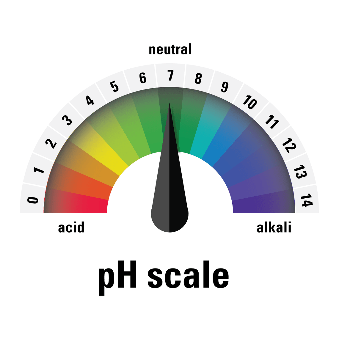
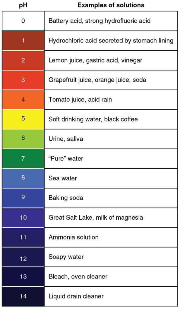
pH is defined as the negative log of the molar concentration of hydrogen ions in a water-based solution. The more abundant the hydrogen, the lower the pH. It’s a log scale, so every unit of pH refers to a 10-fold change in the concentration of hydrogen ions.

Both very low (acidic) or very high (basic) pH can be caustic. But having a low or high pH doesn’t mean it will burn your skin or clothes right away, it might just be a bit unpleasant. But at the extreme ends, protection is needed.

Why is pH Important in Spray Mixtures?

In spraying, the main effect of pH is on the pesticide’s solubility. Solubility matters when mixing and becomes important during cleanout as well.

A minor effect on pH, at least for herbicides, is on chemical breakdown, usually through hydrolysis, when the pH is too high. The effect on breakdown is rarely meaningful during any given spray day, but may play a role if a spray mix is stored overnight or longer.

The Basics: Strong vs Weak Acids

Strong acids like hydrochloric acid (HCl) ionize completely in solution. When added to water, only H⁺ and Cl^– are present, there is no HCl. The water’s pH does not affect solubility of a strong acid.

But weak acids do not completely ionize. The water pH affects the degree of ionization and therefore solubility.

Most herbicides are weak acids. A weak acid is one that does not dissociate completely in solution. A typical example of a weak acid functional group is carboxylic acid (-COOH). In solution, compounds with a carboxylic moiety exist in an equilibrium, with some as -COOH (containing the hydrogen, also called “protonated”) and others as -COO^– and H⁺. In the dissociated form, the acid is more water soluble than in its protonated form due to the negative charge that makes it ionic.

Weak acids have a dissociation constant known as the pKa. When the solution is at the molecule’s pKa, the acid is 50% dissociated. When the solution has a lower pH than the pKa, there is less dissociation and the protonated forms of the molecule dominate. That has two important implications for herbicides.

the molecule becomes less water-soluble at lower pH
the molecule has fewer opportunities to interact with positively charged items

pH Dependent Solubility

Water-solubility is a two-edged sword. On the one hand, having a highly water soluble product makes it easier to dissolve in water. This pays dividends when mixing a batch or cleaning a sprayer because a product formulated as a solution will easily go into a true solution and will stay mixed. Examples are glyphosate, glufosinate, and salts of 2,4-D, MCPA, and dicamba.

On the other hand, most pesticides need to enter a plant to reach their site of action. And a plant cell, with its waxy cuticle and oily membranes, creates an effective barrier for water, and for water-loving molecules dissolved in it. As a result, a formulation that allows the water-soluble product to interact with an oily barrier is needed.

The products that can do this are surfactants. Acting like detergents, surfactants have regions in their structure that are oil-loving (lipophilic) and other regions that are water-loving (hydrophilic). Surfactants can therefore bind to both oil and water and provide a bridge for water-soluble products across oily barriers.

That’s also one of the reason that the most water-soluble products such as glyphosate and glufosinate contain a lot of surfactants in their formulation, reducing the concentration of active ingredient in the jug and possibly leading to foaming with agitation.

Pesticides have a wide range of solubilities, and for some, water pH will play an important role. Below is a table of some water solubilities of selected herbicides.

				Solubility (ppm)
Trade Name	Active Ingredient	Mode of Action Group	pH ~ 5	pH ~ 7	pH ~ 9
Select	clethodim	1	53	5,450	58,900
Ally 2	metsulfuron	2	550	2,800	313,000
Express	tribenuron	2	48	2,040	18,300
Pinnacle	thifensulfuron	2	223	2,240	8,830
Everest	flucarbazone	2	44,000	44,000	44,000
Simplicity	pyroxsulam	2	16	32,000	13,700
Frontline	florasulam	2	0.1	6	94
Varro	thiencarbazone	2	172	436	417
Raptor	imazamox	2	116,000	>626,000	>628,000
Pursuit	imazethapyr	2	2,570	12,870	7,500
2,4-D	2,4-D salt	4	29,934	44,558	43,134
dicamba	dicamba salt	4	>250,000	>250,000	>250,000
Roundup	glyphosate	9	>500,000	>500,000	>500,000
Liberty	glufosinate	10	>500,000	>500,000	>500,000
Heat	saflufenacil	14	30	2,100	>5000
Distinct	diflufenzopyr	19	63	5,900	10,550
Infinity	pyrasulfatole	27	4,200	69,100	49,000

Compare the solubility at pH 7 to that at pH 5. For most of these herbicides, water solubility is worse at lower pH. That is because they are more protonated and become more lipophilic.

I’ve placed a lot of Group 2 products in this table because those products are most often implicated in tank cleanout issues. All Group 2 products in this table, with the exception of Everest (flucarbazone-sodium) have lower solubility at pH 5 than they do at pH 7. For some, like pyroxsulam and floarsulam, it’s a big change. Those products, when acifified, are prime candidates for poor mixability and poor cleanout.

When it comes to dicamba, low pH has another side-effect. It makes the molecule more volatile, increasing danger to sensitive plants nearby. For that reason, acidification of dicamba in its Xtendimax and Engenia formulations is not permitted.

Note that the Group 4 examples, 2,4-D salt and dicamba salt, as well as glyphosate and glufosinate, are highly water-soluble and pH has very little effect on that.

Particularly for glyphosate, the claim that it becomes more oily at low pH and will therefore be taken up more easily, is not supported by these data. Considering that the most acidic pKa for glyphosate (it has four acidic groups) is 0.8, pH would need to be much lower for any noticeable impact on oilyness.

Tank Mixability

Given today’s environment of herbicide resistance, applications with multiple mode of action tank mixes are very common. Acidifying a spray mix to benefit one herbicide may create problems for its tank mix partners.

If there is a concern that spray water is too alkaline, it is recommended that the pH of the finished spray mix be measured. Since many herbicides are weak acids, they will lower the pH of the mixture by themselves. For example, the addition of glyphosate to water with pH 7.5 will drop the pH to about 5 or so, depending on the water’s buffering capacity.

As a result, glyphosate tank mix partners that are pH sensitive may suffer in the presence of glyphosate, and pH may actually need to be raised.

pH Dependent Half-life

Herbicides

There are a lot of claims that pesticides break down rapidly in alkaline spray water. And yet, in my career working primarily with herbicides, I do not recall this ever being a problem in practice.

Below is a table of herbicides for which I could find half-life information, with the help of this comprehensive list produced by Michigan State University.

Product	Active ingredient	Half Life
Atrazine	atrazine	More stable at high pH
Banvel	dicamba	Stable at pH 5 – 6
Bromoxynil	bromoxynil	pH 5 = 34 d; pH 9 = 1.7 d
Fusilade	fluazifop-p-butyl	pH 4.5 = 455 d; pH 9 = 17 d
Liberty	glufosinate-ammonium	Stable over wide range of pH
Gramoxone	paraquat	Not stable at pH above 7
Reglone	diquat	pH 5 = 178 d; pH 7 = 158 d; pH 9 = 34 d
MCPA	MCPA	pH 9 = < 5 days
Poast	sethoxydim	Stable at pH 4.0 to 10
Princep	simazine	pH 4.5 = 20 d; pH 5 = 96 d; pH 9 = 24 d
Prowl	pendimethalin	Stable over a wide range of pH values
Roundup	glyphosate	Stable over a wide range of pH values
Treflan	triflularin	Stable over a wide range of pH values
2,4-D	2,4-D	Stable at pH 4.5 to 7

Note that all of the herbicides are relatively stable. Some are a bit less stable at high pH, but none of the listed herbicides is in danger of breaking down on the day it is being applied. Only one is actually unstable at high pH – paraquat, a herbicide no longer registered in Canada and resticted in many other countries. Those with short half-lives experience them at quite high pH which are rarely seen in practice.

Insecticides

Insecticides are a different story. Several are very sensitive to pH. This table is again adapted from a comprehensive list published by Michigan State University, here.

Trade Name	Active Ingredient	Half-life
Admire	Imidacloprid	Greater than 31 days at pH 5 – 9
Agri-Mek	Avermectin	Stable at pH 5 – 9
Ambush	Permethrin	Stable at pH 6 – 8
Assail	acetamiprid	Unstable at pH below 4 and above 7
Avaunt	indoxacarb	Stable for 3 days at pH 5 – 10
Cygon/Lagon	dimethoate	pH 4 = 20 hrs; pH 6 = 12 hrs; pH 9 = 48 min
Cymbush	cypermethrin	pH 9 = 39 hours
Diazinon	phosphorothioate	pH 5 = 2 wks; pH 7 = 10 wks; pH 8 = 3 wks; pH 9 = 29 days
Dipel/Foray	b. thuringiensis	Unstable at pH above 8
Dylox	trichlorfon	pH 6 = 3.7 days; pH 7 = 6.5 hrs; pH 8 = 63 min
Endosulfan	endosulfan	70% loss after 7 days at pH 7.3 – 8
Furadan	carbofuran	pH 6 = 8 days; pH 9 = 78 hrs
Guthion	azinphos-methyl	pH 5 = 17 days; pH 7 = 10 days; pH 9 = 12 hrs
Kelthane	dicofol	pH 5 = 20 days; pH 7 = 5 days; pH 9 = 1hr
Lannate	methomyl	Stable at pH below 7
Lorsban	chlorpyrifos	pH 5 = 63 days; pH 7 = 35 days; pH 8 = 1.5 days
Malathion	dimethyl dithiophosphate	pH 6 = 8 days; pH 7 = 3 days; pH 8 = 19 hrs; pH 9 = 5 hrs
Matador	lambda-cyhalothrin	Stable at pH 5 – 9
Mavrik	tau-fluvalinate	pH 6 = 30 days; pH 9 = 1 – 2 days
Mitac	amitraz	pH 5 = 35 hrs; pH 7 = 15 hrs; pH 9 = 1.5 hrs
Omite	propargite	Effectiveness reduced at pH above 7
Orthene	acephate	pH 5 = 55 days; pH 7 = 17 days; pH 9 = 3 days
Pounce	permethrin	pH 5.7 to 7.7 is optimal
Pyramite	pyridaben	Stable at pH 4 – 9
Sevin XLR	carbaryl	pH 6 = 100 days; pH 7 = 24 days; pH 8 = 2.5 days; pH 9 = 1 day
SpinTor	spinosad	Stable at pH 5 – 7; pH 9 = 200 days
Thiodan	endosulfan	70% loss after 7 days at pH 7.3 to 8
Zolone	phosalone	Stable at pH 5 – 7; pH 9 = 9 days

Among insecticides, dimethoate, amitraz, and malathion stand out as breaking down rapidly in alkaline water. For these products in particular, it may be important to acifify the spray mix if there is any delay in spraying.

Recommendations

I’ve never been a fan of messing with solution pH unless recommended on the product label. Even when there is evidence that lower pH improves efficacy, consider the impact on tank mix partners.

We’ve seen improvements in solubility and tank cleranout of Group 2 products with raised pH, and ammonia is the most cost-effective way to achieve that. But again, following label recommendations is strongly recommended. The consequences of changes in pH, particularly acifification, can be very detrimental. To be safe, consider doing a jar test before committing to a whole tank to a pH adjustment.

April 2, 2026

How to Interpret a Water Quality Test Result
It’s common advice: Test your water before using it as a spray carrier. You dutifully sample the well or dugout and await lab results. And what comes back is a whole lot of numbers. How to make sense of it all?
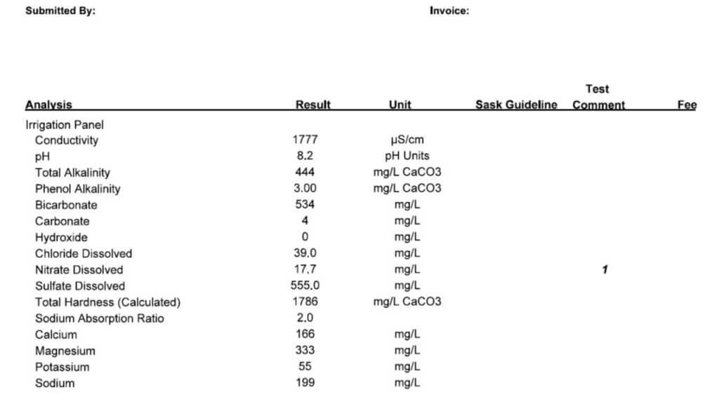
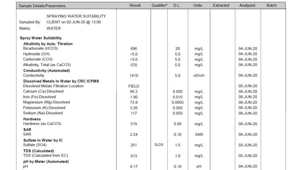
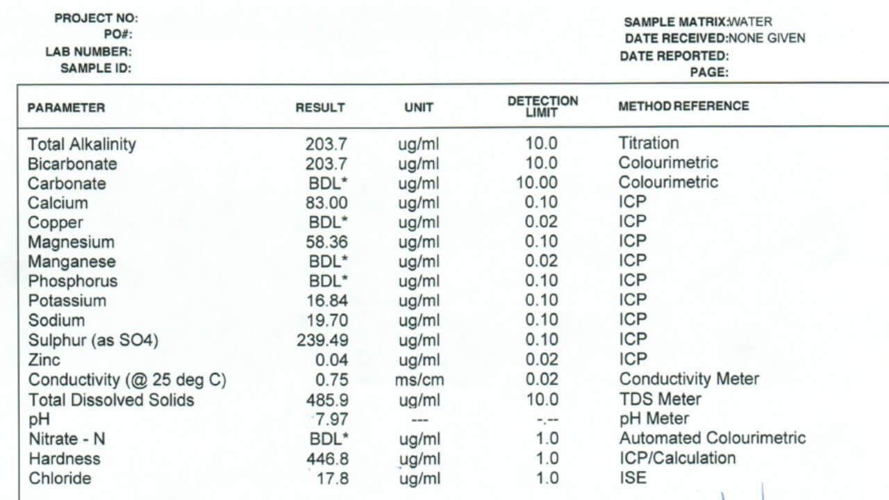
Three examples of water test results conducted by labs in Canada
All three of these tests report a large number of properties and identify specific minerals and other solutes. Which ones are important in spraying? Here is the order in which I look at the numbers.
Conductivity: This property is usually expressed as micro Siemens per cm (µS/cm) and simply identifies how many ionic solutes are in a sample (watch for alternate units such as mS/cm and convert if necessary). It doesn’t differentiate between any minerals or other molecules, and therefore has limited information. But it does tell us if there is a large or small issue with water quality. If conductivity is below 500 µS/cm, the water is probably good for spraying. If the value is around 1000 to 2000, further investigation is necessary. Some water samples return conductivity of more than 10,000 µS/cm, and it’s important to identify which salts are causing that problem.
Note that Total Dissolved Solids (TDS) are often listed, and these are related to conductivity. A common way to get TDS is to multiply conductivity by 0.65. The conversion factor depends on which salts are dissolved but the bottom line is that TDS and conductivity are closely related.
Bicarbonate: Bicarbonates are HCO₃ and their concentration is measured in milligrams per Litre (mg/L), which is the same as parts per million (ppm). Bicarbonates can antagonize Group 1 modes of action and the common threshold is 500 ppm. Research at NDSU has shown that Urea -Ammonium-Nitrate (UAN or 28-0-0 liquid fertilizer) can reduce bicarbonate antagonism in some Group 1 herbicides.
Bicarbonates are negatively charged and are associated with a positive ion, often the hard water cations sodium (Na), calcium (Ca) or magnesium (Mg). As such, waters that are high in bicarbonates are often also hard.
Total Hardness (calculated): This is one of the important parameters. Hardness antagonizes most weak acid herbicides, most importantly glyphosate and g;ufosinate, and also ties up surfactants and emulsifiers which can result in problems with mixing and compatibility. Hardness is caused by metal cations, in order of strength these are iron (Fe⁺⁺), magnesium (Mg⁺⁺), calcium (Ca⁺⁺), sodium (Na⁺), and potassium (K⁺). Of these, Mg and Ca are typically most abundant, although some water is high in Na.
The Total Hardness (ppm) reported in water tests is done by taking the most common two cations, calcium and magnesium, and using this formula: 2.497*Ca + 4.118*Mg. Note that some tests report hardness in Grains per Gallon, in this case, multiply grains by 17.1 to get ppm.
While this calculation usually gives an accurate prediction of hardness, you may need to have a look at iron and sodium as well. Iron is less common, but some well waters are high in sodium or potassium. These minerals are not captured in the Total Hardness measurement. A water test low in Total Hardness may still be high in sodium, these are typically the samples with high conductivity.
The threshold for Total Hardness depends on the herbicide, its rate, and the water volume. The most common quoted values are 350 ppm for the lower rates of glyphosate (1/2 L/acre equivalent), and 700 ppm for the higher rates. Lower water volumes increase the concentration of herbicide, and reduce the impact of water hardness or bicabonates.
pH: This parameter is a bit over-rated because it is later affected by the herbicide and adjuvant dissolved in it. There is usually no concern with pH between 6 and 8, and water is rarely outside this range. It is best not to change the pH of water unless it is required on the label for mixing, because some products require low, and others require high pH for optimum solubility. Compatibility is an ever greater concern as our tank mix complexity increases.
Water Conditioners
The most common water conditioner is ammonium sulphate [AMS, (NH₄)₂ SO₄]. In its pure form (21-0-0-24), a concentration of 1% to 2% w/v (8 to 17 lbs AMS/100 US gallons of spray water) solves most hard water and bicarbonate issues. Be cautious of using too much AMS (>3%), when added at high concentrations to some herbicides it can burn crops.
Research has shown that AMS works in two ways: The sulphate ion binds with hard water cations, forming an insoluble precipitate that prevents the antagonistic cations from binding to, and inhibiting, the herbicide. The ammonium ion has been shown to improve cellular uptake by weak ion herbicides.
Some product labels call for UAN as an adjuvant. UAN contributes ammonium, but not sulphate ions. As a result, while it may improve herbicide performance, it does not remove antagonizing cations from the mixture.
Acids have been used to combat hard water. Most common herbicides are weak acids, and the acid constituent, usually a carboxilic acid, has a unique pKa. The pKa is the pH at which half the molecules are protonated (contain a hydrogen atom, resulting in an uncharged acid constituent) and the other half are not protonated (negatively charged). If the spray mixture has a pH below the pKa, the weak acid herbicides become protonated. This means the herbicide becomes less water-soluble, but also that it has less chance of interacting with a hard water cation. Acids that work in this way are less effective at ameliorating the effect of hard water than AMS.
A small group of acids that includes citric acid and sufphuric acid can sequester or bind with hard water cations. But they do not contribute the ammonium ion that assists in weak acid herbicide uptake.
If your water is questionable for spraying, there are four common choices:
- Select a different well or dugout
- If the problem is barbonates or hardness, treat water with a conditioner such as Ammonium Sulphate (AMS), available in pure form as 21-0-0-24. Some acids (citric, sulfuric) can form conjugate bases with hard water cations, removing them from solution. But the associated significant lowering of pH should be treated with an abundance of caution as it may affect solubility of some pesticides.
- Reduce water volumes or increase herbicide rates.
- Use a municipal treated water source or invest in a reverse-osmosis (RO) system. RO is neither cheap nor fast and requires additional investment in storage, and a way to deal with solute-enriched waste water. But it may be the best option for some.
An Ammonium Sulphate calculator, originally developed by Winfield United using data from NDSU, can be downloaded here:
AMS-Calculator-Sprayers101-1 Download
An excellent resource for adjuvant and water quality topics is this addendum in the North Dakota State University Guide to Weed Control.
Using good quality water lowers the likelihood of problems with mixing and overall performance and that pays significant dividends later.
April 1, 2026
Wanted: A New Technology for Assessing Spray Coverage – The Spray Doctor
“If you can’t measure it, you can’t improve it”. While the source is nebulous (Peter Drucker, Lord Kelvin, or Antoine-Augustin Cournot), the sentiment is clear.
The status quo
In the world of crop protection, considerable resources are expended to distribute a pesticide over a target. And yet, sprayer operational settings and spray coverage are rarely assessed. As a result, too much time elapses between the application and observing the biological results to evaluate and correct equipment performance. The damage (be it waste or an inconsistent and sub-lethal dose) is done. All sprayer operators know this to be true, so why do precious few perform these assessments?
Perhaps, dear reader, you have personal experience assessing coverage and already know the answer. Perhaps you’ve performed the iterative dance that is placing, spraying, retrieving, assessing and re-placing water sensitive paper (WSP). Perhaps you’ve sprayed fluorescent tracers and hunted for faint glows at twilight using UV lights. Perhaps you’ve looked for residue from diatomaceous earth or fungicides. Or, perhaps, you’ve trusted in the falsely-comforting “shoulder check” and assumed dripping must mean you’ve hit the target.
Existing methods are complicated, subjective, messy and time-consuming. We need an alternative.
The alternative
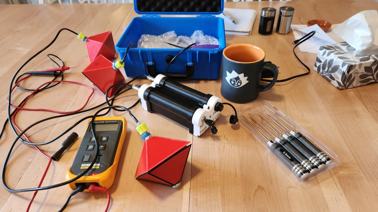
Consider a permanent, solar-powered sensor that supplies real-time spray coverage data to your smartphone via a cellular connection. The output could be visualised in a simple and intuitive way, and immediately available to both sprayer operators and farm managers. If the sensor was relatively inexpensive, sufficiently hardy, and easy to deploy, its utility would only be limited by your imagination:
- Stakeholders could confirm the correct functioning of their equipment before committing to the application. Decisions could be made to change operational settings, repair equipment, or delay until conditions improved.
- The sensors would provide coverage data specific to their location and orientation. Units could be installed in difficult-to-spray regions such as treetops, or canopy-centres, or fruiting zones. Sensors could be placed where pest/disease pressure has been historically high, or where wind is a known issue.
- Large operations could install them in a test-row, where sprayer operators would perform a gauntlet-style calibration run prior to a day of spraying.
- Spray records could inform compliance audits, supplement insurance or CanadaGAP traceability requirements, or be used in agronomic assessments.
In 2025 I was approached by an Australian developer who claimed he had a device that did all of this. And, if that weren’t enough, it could also monitor certain meteorological factors such as pre-spray moisture levels and temperature and report post-spray evaporation rates. I could barely contain my excitement. A prototype was in my hands a few weeks later.
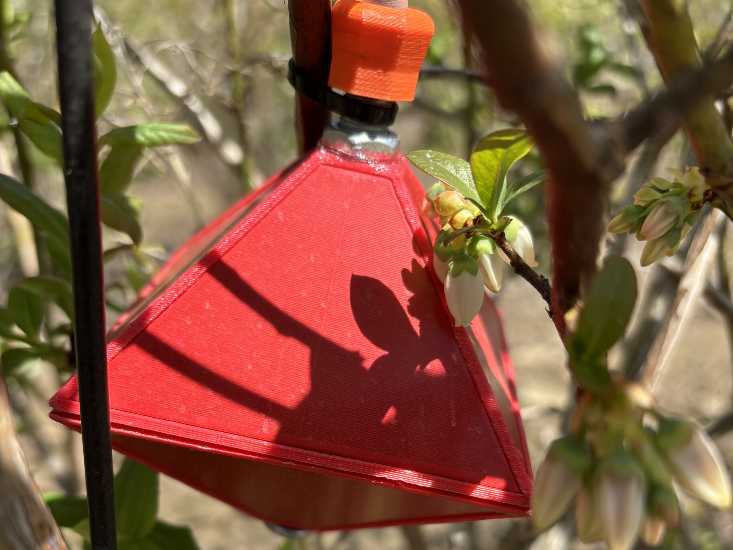
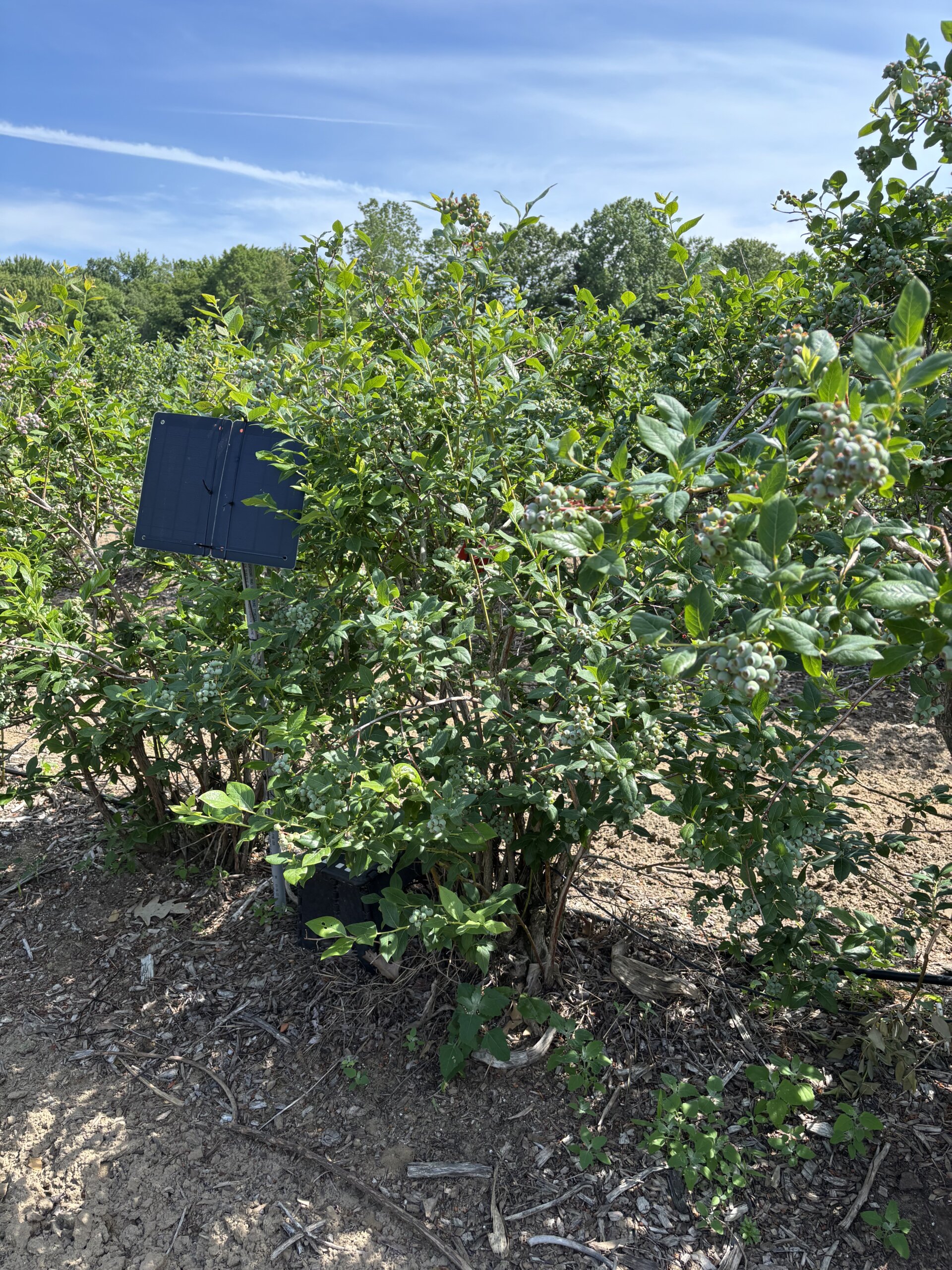
Prototype, 8-sided sensor located in a blueberry bush.
Solar panel powering three, 8-sided prototype sensors spanning 10 meters of highbush blueberry.
Benchmarking the sensor
The Spray Doctor (working name for the prototype) started its life as a leaf wetness sensor, evolving into a spray coverage sensor piloted in 2023/24 in Australian and New Zealand grape production. The history of earlier iterations and company schisms is convoluted, and fortunately immaterial to our purposes. All I needed to know was that we weren’t starting from scratch. Several of the questions regarding how accurately the surface could detect spray deposition were already addressed by independent research.
The sensing surface is impregnated with an array of capacitive wetness sensors. The sensor responds to the surface area covered and not deposit density. Researchers reported a reliable response range between ~10% and 50% surface coverage. Given the arguable “ideal” coverage standard of 10-15% surface area, this includes the range of interest for most sprays.
Benchmarking against WSP was part of the foundational assessment. A droplet of water deposited on WSP produces a high angle of contact and very little spread, while the same droplet deposited on plant tissue tends to produce a lower angle of contact and more spread. This means the stain produced on WSP is smaller than would be produced on plant tissue, depending on how smooth, vertical or waxy the tissue surface was.
It was therefore surprising that WSP were found to report a higher degree of spray coverage during water-only sprays than the sensor. It seemed droplets more easily coalesced and ran off the sensor surface. This was ultimately interpreted as an advantage, because the sensor would better emulate how a leaf surface would respond to the influence of surfactants and spray quality.
Adding a surfactant to a spray solution improves droplet adherence, and/or reduces surface tension, improving the degree of contact on plant surfaces. Likewise, it was found that surfactants increased the degree of coverage reported by the sensor, and when actual chemistry was sprayed (e.g. sulphur powder or copper sulfate) there was an effect on the degree of coverage reported. This is unlike WSP, where adjuvants and chemistry do little to increase the spread.
And so, like every method for assessing spray coverage, the sensor has limitations and caveats. If you have some doubt as to the sensor’s accuracy, do not get distracted by the fine detail. Remember, most operators currently have no feedback whatsoever; even a binary response (e.g. hit or miss) would be welcome. The sensor is sufficiently sensitive and consistent to resolve coverage in a range relevant to most sprays, and therefore worth field testing.
The experiment
My role in this story was to work with a grower to evaluate the sensor’s ability to report coverage information in a clear and actionable way. There were three questions:
- Does data from the sensor influence a sprayer operator’s behaviour?
- Does that change in behaviour lead to improved spray coverage (implying more efficient and effective crop protection).
- Could we “dial in” the hardware and the interface based on the grower’s feedback?
In part two, we share our experience installing and using the Spray Doctor, as well as supply answers to these questions. Stay tuned.
Thanks to Brandon Falcon (Falcon Blueberries) for volunteering his time and farm for this evaluation, and the developer for the in kind donation of the prototype Spray Doctor.
January 23, 2026
Evaluating the return on investment of optical sprayers for horticulture
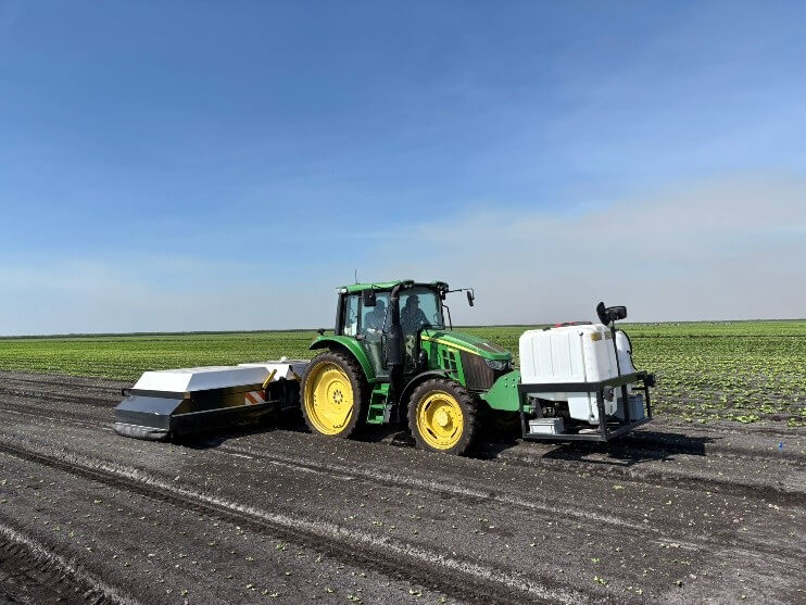
Investing in an optical sprayer for horticulture is not a straightforward financial decision. Compared with a conventional boom sprayer, the upfront capital cost is substantially higher, often by an order of magnitude, and most commercial systems require an annual software or service subscription to operate. Despite these barriers, adoption is accelerating, and many growers who have made the investment report very positive outcomes.
To help clarify when and where this technology makes financial sense, I developed a calculator to estimate the return on investment (ROI) of optical sprayers under a range of production scenarios. The goal of this tool is not to promote the technology, but to provide growers and advisors with a structured way to evaluate whether it fits their specific operation.
Note: This calculator was designed for onion and carrot production in Ontario, Canada. Model parameters can easily be adjusted reflect other production systems. However, if you need assistance making these changes you can contact me by email.
How to use the calculator
At first glance, the calculator may appear overwhelming. It contains many data points and requires a fair amount of information to be entered. This level of detail is intentional: the objective was to strike a balance between simplicity and realism, avoiding oversimplification that could lead to misleading conclusions.
The calculator runs directly in your web browser, and nothing needs to be downloaded or installed. Results update automatically as you type. The values you enter are saved only in your own browser, so they will still be there the next time you open the calculator on the same device. They are not sent to or collected by Sprayers101.
Every input field and every result has a short explanation. Hover over it, or tap it on a phone or tablet, to see what it represents. Labels with a dotted underline have an explanation. Each section also has a ? button beside its title, which opens a more detailed description of what the section does and how its inputs affect the results.
Inputs
Enter your information in five panels:
- Report details (optional): name, company and date for the downloaded report.
- Sprayers cost and capacity: purchase prices, subscription, tractor cost, maintenance and field capacity.
- Your crops: area, yield, expected yield increase, sale price, harvest cost and hand weeding hours.
- Herbicide programs: price, weed cover, applications and rates for each product. Products can be added or removed.
- Financing (optional): needed only for NPV, IRR and loan payments.
A switch at the top converts all inputs between metric and Imperial (US) units.
Results
The results panel shows the net annual benefit of the optical sprayer, where it comes from, and the payback period and return on investment.
Three tables follow:
- Financial metrics: payback, ROI, NPV, IRR and loan payments in one place.
- Sensitivity analysis: how the results change with different areas of the two crops. The colour bands are for reference only and do not represent any standard.
- Conventional vs. optical: both sprayers side by side, per year.
Download results creates a printable report, and Reset restores the example values.
Default Values
The calculator is pre-filled with generic values from grower discussions and informal benchmarks. They are placeholders for general reference only and are not accurate enough to support financial decisions. The output is only as good as the inputs, so replace the defaults with your own operation’s data.
Insights from scenario testing
Even using rough approximations, several consistent patterns emerge from adjusting the calculator inputs:
Herbicide savings alone rarely justify the investment
In high-value horticultural crops, herbicide costs are often a relatively small portion of total production costs compared with labor, equipment, and the overall value of the crop. In many cases, any reduction in herbicide expenditure is largely offset by increased tractor hours resulting from slower operating speeds and narrower effective spray widths typical of optical sprayers.
Labor savings can be decisive
When the technology results in meaningful reductions in hand-weeding, the financial impact can be substantial. This is especially true in crops such as onions, where hand-weeding is both costly and difficult to source reliably. In these situations, labour savings alone can drive a favorable ROI.
Yield protection may outweigh cost savings
Several growers report stand losses and weakening associated with herbicide phytotoxicity as a major production risk. By limiting spray exposure to crop plants, optical sprayers can significantly reduce or even eliminate this issue. In high-value systems, relatively small yield gains resulting from improved crop safety can translate into revenue increases large enough to justify the technology, even if other savings are modest.
Scale matters
When evaluating advanced sprayer technologies, scale becomes a decisive factor. The high capital investment and ongoing service fees may be difficult to justify for small, and in some cases, even medium-sized operations.
What about herbicide resistance?
The long-term implications of optical sprayers for herbicide resistance management are still uncertain. Recent research from the University of Arkansas has raised concerns in field crop systems, suggesting that poorly optimized optical spraying can result in short term gains, but these can be outweighed over time by higher weed escape rates compared with broadcast applications. If these escapes are allowed to grow and set seed, rapid seedbank replenishment and accelerated resistance development may occur.
This highlights an important limitation of short-term ROI calculations. A single-year economic benefit may look attractive, but if the system allows even a small number of weeds to consistently escape and reproduce, the long-term consequences can be severe.
On the other hand, optical sprayers may eventually enable new resistance-management strategies. It is possible that new active ingredients, higher labelled rates, or novel use patterns could be registered specifically for targeted spraying in horticultural crops that would not be feasible with broadcast applications. Such developments could significantly improve resistance management tools. As always, it is essential to remember that the label is the law: only registered products and rates may be used, regardless of perceived crop safety.
ROI implications beyond herbicide spraying
Optical sprayers can deliver value beyond herbicide applications, even though weed control is their primary use. These additional uses may improve overall ROI. However, because their economic impact is still difficult to quantify, they have not been included in the calculator.
Depending on the model, additional value-generating capabilities can include:
- Creation of weed maps: Some systems can generate weed maps automatically while spraying, at no additional operational cost. These maps can support future management decisions.
- Application of fertilizers and other pesticides: Although optimized for herbicides, optical sprayers may also be used to apply other inputs, such as fertilizers or non-herbicide pesticides.
- Crop thinning: Certain manufacturers have developed algorithms for automated crop thinning, particularly in crops like lettuce.
Conclusion
Even using approximate inputs, it is clear why optical sprayer adoption is expanding rapidly in Canada.
- For medium to large-scale operations, the ROI can be highly attractive, and the range of potential benefits continues to grow.
- As the technology matures, more equipment options are emerging to serve a wider diversity of crops and farm sizes.
- Manufacturers are introducing wider and more flexible platforms, and Ontario-based companies are actively developing alternative machines and service-based business models that may better suit smaller operations.
It is difficult to argue that optical spraying is a passing trend. While it’s not a universal solution and must be implemented carefully, the technology is clearly here to stay. It will reshape weed management and production economics over the long term.
January 16, 2026
The Micothon M2 – The Benefit of Air-assist Spraying in a Vegetable Greenhouse
I’ve experienced a few spectacular failures trying to build niche sprayers. Until now, I haven’t had a reason to write much about them. But I decided the contrast, and confession, would be a fun way to set the scene for a discussion about an excellent niche sprayer.
Failed Attempts
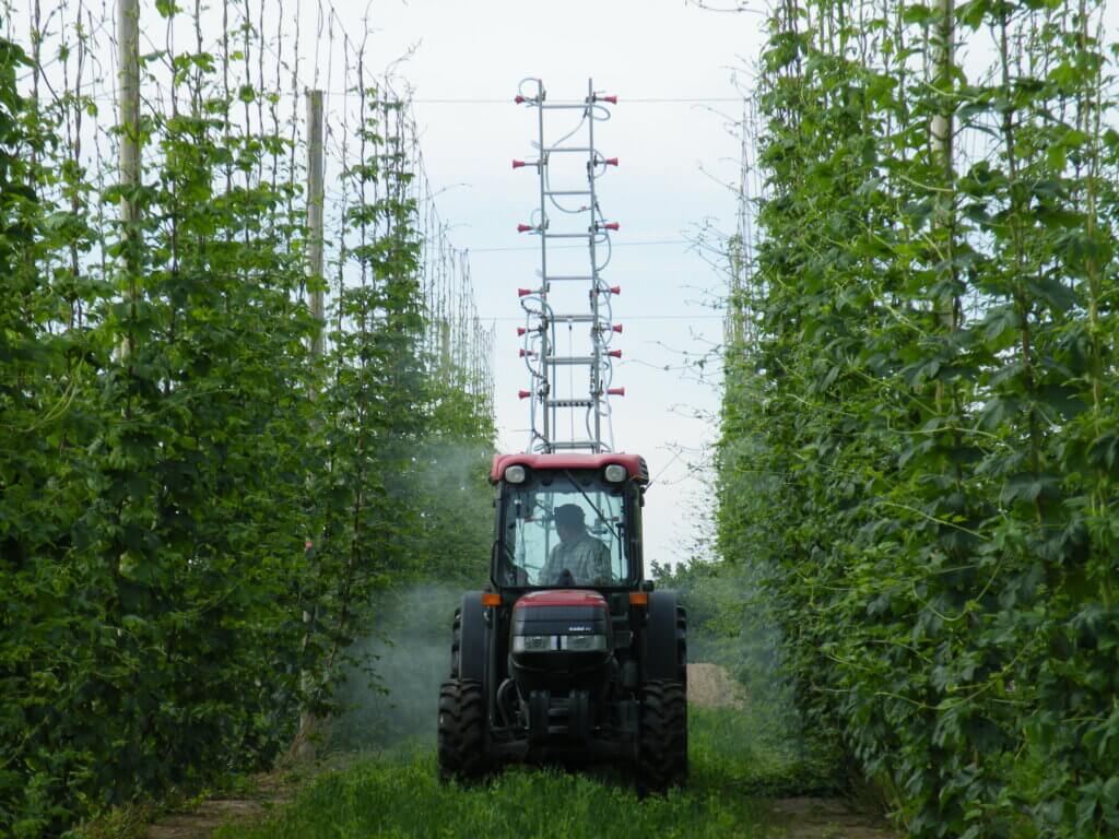
First, the ill-fated “Hops Sprayer”. We used an adjustable ladder to position 20 feet of arborist guns between hop rows. The nozzles could be raised and engaged to match the growing crop canopy. While it left decent coverage on the adaxial surfaces, we quickly realized it needed air-assist to get under the leaves and battle high winds at the top of the trellis. It’s since been cannibalized for parts, and the rusted remains haunt me whenever I drive by the outdoor storage area at our ag research station.
The Hops Sprayer. A 3 point hitch, vertical boom that could adapt to match canopy height.
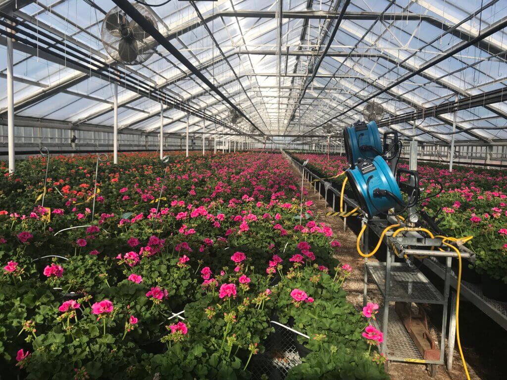
Later, encouraged by a minor success ducting a backpack mist blower with PVC and Coroplast, I tried building an air-assisted spray cart for a floriculture operation. It featured commercial, high-volume radial fans paired with hollow cone nozzles positioned in front of the air outlets. With respect to GreenTech and Croplands Equipment in Australia, I tried to build a bargain-basement SARDI-style head.
When it wasn’t threatening to tip over, it managed decent coverage over almost 2 meters. Almost.
As it turns out there’s a very good reason engineers use computational fluid dynamics to design air-assisted sprayers. We were ultimately beaten by an uneven greenhouse floor crowded with obstacles, a stiff canopy of geraniums, and the inverse square law, which states: “The farther away an object is from an effect, the less change can be observed in the object”. This rig now has a new life circulating hot air in a boiler room.
And I once built an air-assisted, tow-behind sprayer to spray troughs of tabletop, hoop house strawberries. That unit laid down an excellent, uniform spray on all foliar surfaces, but it was frustrating to use. There was almost no clearance in the hoop house, which changed height with the topography, and the alternator couldn’t keep the battery sufficiently charged to run the pump and fans. I felt we could overcome these small difficulties, but sadly the operator ended this experiment halfway through the season. I can only assume the sprayer is now an interesting piece of lawn sculpture.
This sprayer had potential, but limited resources prevented it from getting beyond the beta stage.
The Micothon M2
Despite my inability to build a decent air-assisted sprayer, I have always maintained that air-assist is the secret sauce for efficient, uniform spray coverage. Lucky for me, Great Lakes Greenhouses (GLG) agreed. No stranger to innovation, the company recently purchased a first generation, air-assisted Micothon M2 greenhouse sprayer and invited me to come see it. This was a proper sprayer designed by engineers, and not a delusional plant physiologist, so I was excited to assess and calibrate it. This article will describe what we learned and perhaps in some small way, validate my failed attempts.
A quick walk around before we got to spraying.
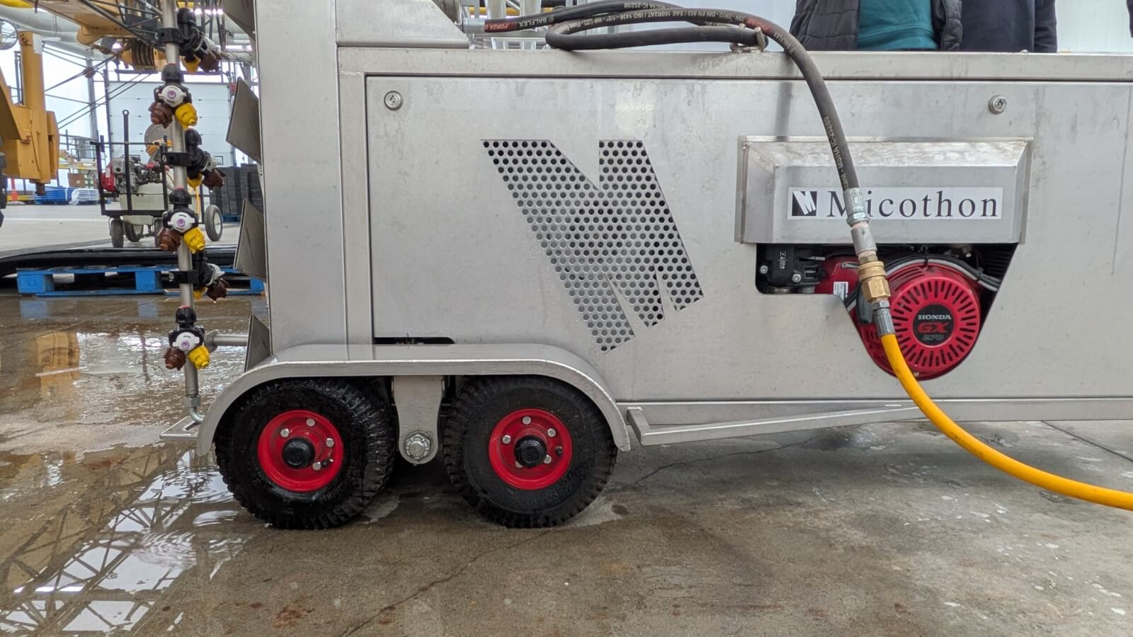
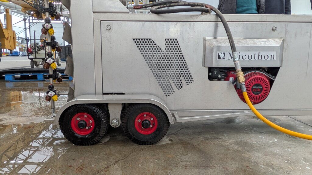
The M2 features a vertical boom design supported by a portable tender unit, but that’s where the similarities to a classic “tree” sprayer end. Rather than riding on the hot water pipes, or tipping onto two wheels like a hand cart, this version rides on self-leveling wheels. It is drive-assisted but still has to be guided by an operator, like a self-propelled walk-behind lawn mower.
Drive-assist, self-levelling wheels.
The mast features 18, three-position nozzle turrets (nine to a side). GLG requested a bespoke spring-loaded break-away section at the top of the boom. This allowed the top nozzles to “duck” under an annoying section of greenhouse infrastructure that would have otherwise prevented it from being positioned between the rows.
A spring-loaded, break-away boom section (with guard) to prevent impact damage.
The break-away section in action.
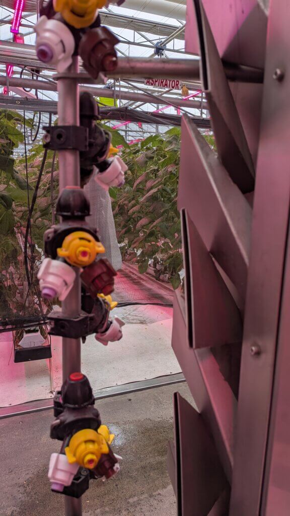
The air is generated by a centrifugal fan powered by a Honda motor. The air travels up the ducted mast to a manifold of narrow air outlets. When the sprayer is moving, the air outlets precede the nozzles, which initially seemed wrong as the spray would be released outside the air stream. But, upon closer inspection, we saw that the air outlets are not only angled up by 45 degrees but are also angled back so the air can transect the spray.
Air outlets and nozzles – front view.
Air outlets and nozzles – side view.
It was suggested that the blade of air acts like an airfoil, creating an area of low pressure and sucking small droplets into the airstream. This is Bernoulli’s principle and it describes how wings create lift. Personally, I think it behaved more like a Venturi. I’m open to debate since, as evidenced by my attempts at building a sprayer, I’m no engineer. What matters is that we didn’t see any droplets hanging in the air as the sprayer passed. It works.
Calibration and Optimization
We followed the same greenhouse sprayer optimization protocol I’ve outlined in this article. Go give it a quick read and come back so I won’t have to reiterate why we took the steps we did.
Travel speed and air settings
The sprayer was set to speed “3” of a possible “5”, as recommended by Micothon. Travel speed dictates dwell time, which is the duration the air is focused on the target. Observers stood in the drive alley and in the two adjacent alleys to see how the air moved leaves. The upward angle of the outlets combined with the volume produced by the centrifugal fan wafted and twisted leaves on their petioles. This created sufficient movement throughout the canopy, but not so much that it caused the canopy to louver shut. It was a Goldilocks situation so there was no need to alter anything.
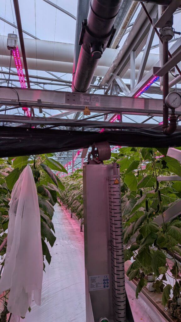
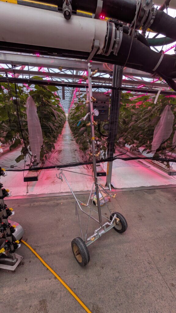
Preparing to guide the Micothon M2 through the cucumbers under red LED lights. This image gives perspective of canopy height, density and the sprayer clearance.
Pressure and nozzles
The tender system regulator was set to 41.5 bar (600 psi) and that pressure dropped to 5.5 bar (80 psi) according to the gauge on the sprayer. While we didn’t test it, I’m certain the pressure at the furthest (aka highest) nozzle would have been closer to 5 bar (~70 psi). With observers in place, we started spraying water using the Albuz 025 (lilac) hollow cone tips.
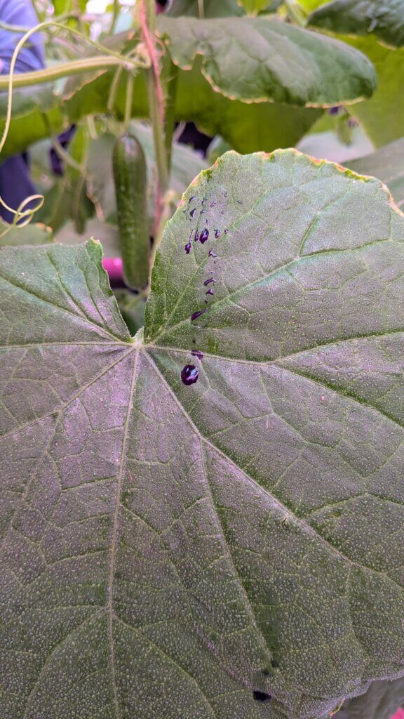
We saw the highest nozzle positions were spraying over the canopies and did not need to be on. We also saw drip points form at the tips of the leaves and the bottom of the cucumbers. There was evidence of yellowed (possibly damaged) tissue at the leaf tips, suggesting they were often sprayed to drip. This is wasteful and tends to redistribute deposits in undesirable ways. While it’s hard to avoid on the waxy, vertical cucumbers, it can be prevented on the leaves.
Note the drip point formed at the bottom of the fruit. This is hard to avoid, but can at least be minimized.
We turned off the top nozzles, swapped to Albuz 02 (yellow) hollow cones, moved to an unsprayed canopy and tried again. Effectively this was a 20% cut in water and product, but there were no more drips on leaves and less evidence of coalescing deposits. The cucumbers still had drip points, but without an adjuvant that was the best we could do. That’s assuming there would be value in spraying the fruit in the first place – these sprays were targeting the foliage.
Coverage
With the subjective part of the assessment complete, it was time to quantify spray coverage. Water sensitive papers were oriented co-planar with the leaves and essentially parallel to the ground. We clipped them 2-3 cm below the leaves by affixing them to the petioles. This way they would move with the leaf and represent a very challenging target (reminiscent of a sucking insect on the abaxial leaf surface).
This is a difficult target to hit. The spray must get up between the leaf and upper side of the water sensitive paper, which is not in line-of-sight of the nozzle.
We divided the canopy into quarters, placing one target in each section. This spanned the height of the canopy, but we also positioned them along the canopy depth: One on each of the four plants in the row. This left us with a diagonal cross-section. Read it again – you’ll get it.
Then we sprayed the row from one side and inspected the results. We saw excellent coverage on the abaxial surfaces of the two plants closest to the sprayer. We expected that. But we were pleasantly surprised to see the spray got in under the umbrella-like leaves and deposited on the adaxial surfaces. This was not line-of-sight for the nozzles, and there wasn’t much room between the paper and the underside of the leaves, so this was clearly the result of air-assisted droplets.
There was also respectable coverage on the two plants on the far side of the row. These targets were greatly improved once we travelled down that alley and saw the cumulative coverage. This is why you should (almost) never perform alternate row spraying.
Abaxial side of the water sensitive papers. From left to right, papers ascended from the lower quarter of the nearest plant to the upper quarter of the farthest plant in the row.
Adaxial side of the water sensitive papers. From left to right, papers ascended from the lower quarter of the nearest plant to the upper quarter of the farthest plant in the row.
Compared to a tree
Since I was in the neighbourhood, we decided to see what a conventional, hydraulic tree could do by way of comparison. Frankly, there was none.
A typical greenhouse tree. Note the 1/4 turn drain near the pressure gauge, the lack of check valves, and the uneven distribution of the nozzle positions (i.e. more at the top) likely intended to direct more flow higher in the canopy.
The tree was nozzled with Albuz 04 (red) hollow cones angled upwards. There were only a few check valves, so it leaked when it was turned off and had to be drained at the end of each row using a quarter turn valve. Coverage was generally excessive (i.e. coalesced droplets and lots of run-off) and non-uniform (we randomly missed both adaxial and abaxial surfaces).
Run-off was so pronounced that it washed the dye off the water sensitive papers.
We re-nozzled to my favourite load out: TeeJet TwinJet fans alternating back and forth by 45 degrees from centre. Using 03’s (blue), we observed improved uniformity, but still saw misses and suspected we were still using too much water. When leaves are drenched they get heavy, causing them to hang lower and obscure the other parts of the plant. This is the contradiction that limits a strictly hydraulic system: Pressure motivates droplet movement, so you need slightly larger drops and more volume. However, too much water causes run-off and weighs leaves down, obscuring the rest of the canopy. Catch 22.
I proposed getting a set of 02 (yellow) tips in the hopes there would still be enough spray for better uniformity. I hope they tried it.
A few beefs about the M2
There’s always room for improvement. Before you think I’m selling these sprayers, here are a few observations from the owners and from what we saw that day. No deal breakers, just some nice-to-haves:
- The diesel exhaust from both the sprayer and the tender cart is not ideal. Applicators wear respirators, and the greenhouse fans tend to dilute the exhaust, but a battery system (perhaps like a drone) would be preferable to power the drive electrically.
- There was a latency with the self-leveling wheels and with air build-up in the tower portion of the sprayer. You simply need to be patient before you start down a row.
- The tower section gets hot to the touch, likely because of the position of the exhaust pipe.
- The alternator on board recharges the battery, but if you let it sit the battery is depleted (sounds like the same trouble I had with my sprayer, which is somehow gratifying).
I’m sure you’re asking “How much?”
Well, at the time of writing, it was almost $70,000.00 CDN, but don’t judge it too harshly! Bear in mind that our assessment saw a reduction of 20% water and crop protection product that would otherwise have ended up on the greenhouse floor. Not only is that a big savings in water and inputs, but it’s fewer refills and it produced far better spray coverage that a hydraulic system. While improved coverage is not always linked to improved efficacy, they certainly go hand in hand. And when we’re considering “softer”, biorational greenhouse chemistries, improved coverage is the best bet we have for pest control.
All in all, this was an excellent sprayer that I hope is the first of many to grace Ontario’s greenhouses.
Thanks to Great Lakes Greenhouses for the invitation, and thanks to all the other grower cooperators (names withheld to protect the innocent) that took a risk on building budget, niche sprayers with me. Sometimes, you just have to throw money at it.
December 8, 2025