Category: Speciality Sprayers

Main category for all sprayers that are not horizontal booms

  • Calibrating a Plot Sprayer for Airblast Crops

    Calibrating a Plot Sprayer for Airblast Crops

    The calibration of handheld plot sprayers is an important part of agricultural research, and this article already covers all the bases… as long as you are spraying broadacre or row crops. But what happens when you are trying to emulate an airblast sprayer and treating a tree, bush, cane or vine?

    The key difference is that spraying a two dimensional area requires the operator to pass the boom over the target at a uniform height and pace to achieve consistent coverage. But, a three-dimensional target requires the operator to circle the target, or spray from both sides, until it has received the required dose (or volume).

    In order to scale down a typical airblast carrier volume for small plot work, we need to know three things:

    1. The area you wish to treat (e.g. bush, grape panel, tree, etc.), including it’s share of the alley (in m2).
    2. The emission rate from the calibrated plot sprayer (in US gal./min.)
    3. The airblast carrier volume you wish to scale down (e.g. L/ha).

    The illustration below shows two options for calculating the treated area. Option A requires you to measure from the outermost edges of the canopy (imagine if the canopy was wet and dripping – the dripline is that outermost point). It is less consistent than the preferred Option B, where the area is determined from row centres and planting distance.

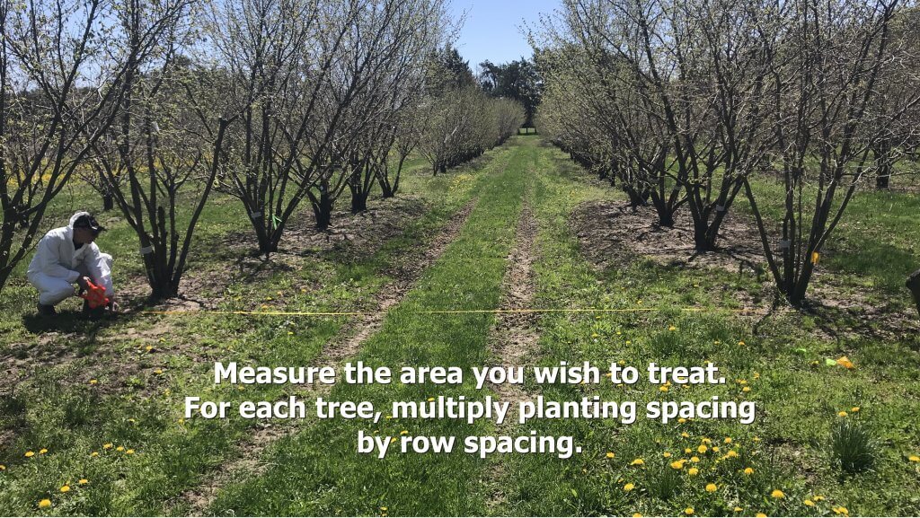
    Two options for scaling down an airblast carrier volume for small plot work. Both produce the same treated area, but Option B is the preferred method.
    Use the average planting distance and row spacing in metres. For a panel of grapes, use the centre of each panel as the planting distance.

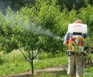
    If you are using a CO2 powered hand wand (preferred over a manual pump) with one or more hydraulic nozzles, then you can calibrate it using the methods in this article. There are battery-powered options from Jacto and Petra Tools, the latter offering a battery powered ULV system as well. Makita also has a battery entry (image below). However, if you are using a backpack mistblower, which better approximates an airblast sprayer compared to a hydraulic hand boom (see this article), it requires a different approach. Plus, you get to look like a Ghostbuster, which is a win in my book.
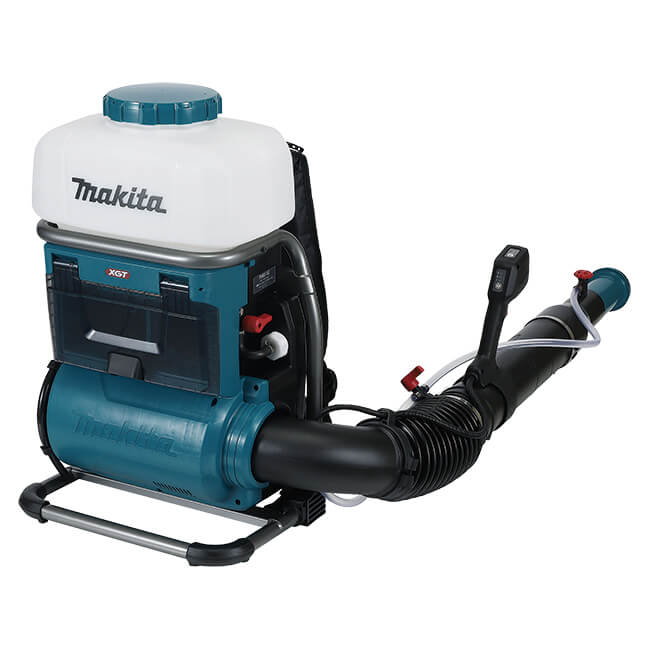
    PM001GL201 – 40V max XGT Brushless Cordless 15L Backpack Mist Blower (8.0Ah x2 Kit)

    Follow along in the following images as we explore how to calibrate a backpack step by step:

    When transporting a mistblower, use a loop of nylon cord to secure the boom in an upright position.
    For calibration, fill the completely empty sprayer with a known volume of water. If the boom is gravity-fed, be sure the feed valve is closed so the water doesn’t run out of the boom.
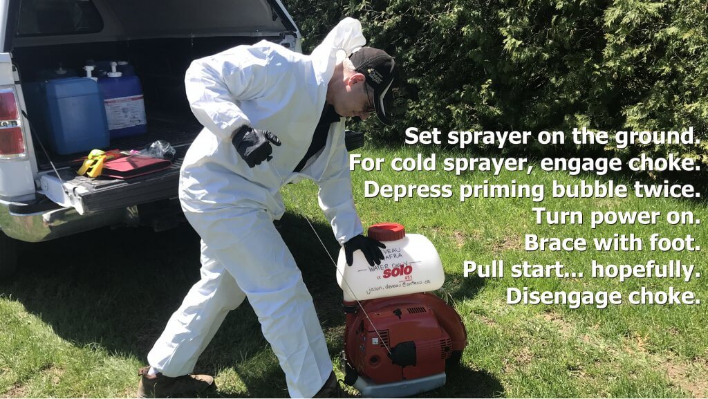
    With the sprayer on the ground, brace it with your foot. Step on the metal frame, not the motor housing or tank. Follow the operating instructions to pull start the motor.
    Being cautious of the hot exhaust, set the sprayer on a tailgate, or other elevated surface to facilitate strapping it on.

    Be aware that most mistblowers use gravity to feed the spray mix from the tank to the boom. A pressure pump kit is recommended for applications where the spray tube is held upward more than 30 degrees to maintain a consistent discharge rate. A hip belt is also recommended to reduce fatigue. Examples are shown below are for Stihl-brand sprayers. Some may or may not require the pump (e.g. Tomahawk) but they are primarily intended for mosquito control and in that case a consistent rate over a vertical plane may not be as important.
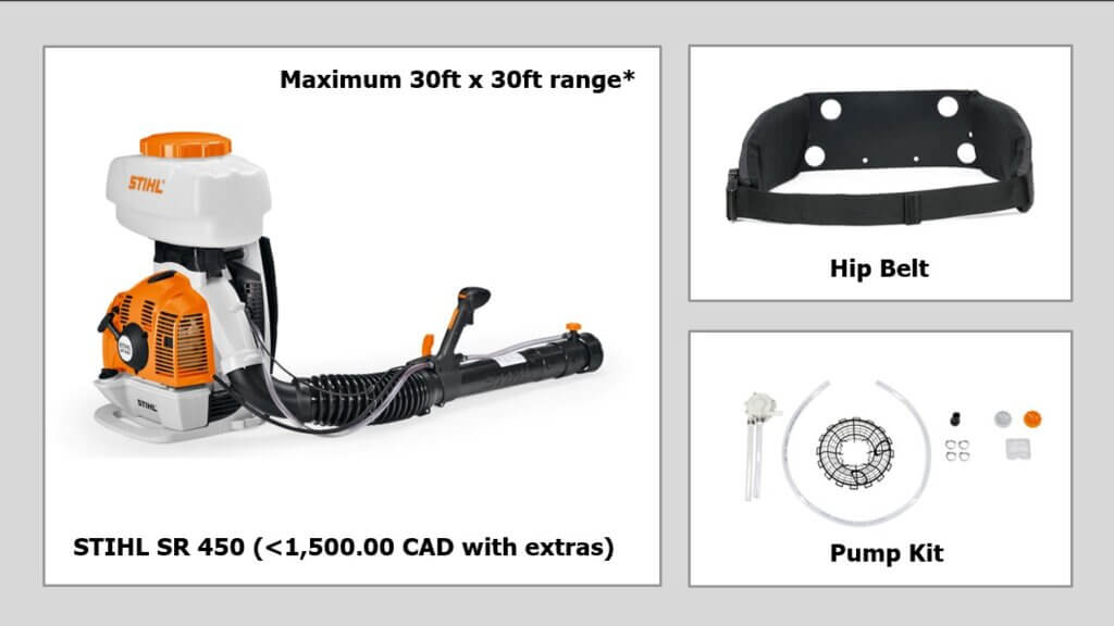
    If your sprayer does not have a pump kit, pointing the boom upward will cause spray to slow or even stop. This greatly diminishes your ability to reach high targets and achieve consistent coverage. In this case, attach the deflector (which comes with the sprayer) before proceeding with the calibration.

    Deflectors angle the spray upwards without having to lift the boom. This is easier on your shoulder and keeps the rate consistent.

    Set the flow rate to the preferred setting (usually a dial at the end of the boom), and using a stopwatch, time how long it takes to spray the entire volume. Be sure to move the boom exactly as you would when spraying the target, either side-to-side or up-and-down, to capture possible rate changes from the gravity feed. Convert the output to US gal./min.

    When timing output, move the boom as you would when spraying the target.

    Alternately, some people will stand on a bathroom scale with the backpack full. Then get off and spray for a period of time. Then get back on the scale. One millilitre of water weighs one gram, so you can calculate the flow from the weight difference.

    Now you know the area and the emission rate. You should have a target carrier volume in mind (e.g. L/ha). Using the following example, let’s determine how long you need to spray the target:

    A sample calibration.

    In this example, an ideal airblast Carrier Volume [C] for the orchard is 400 L/ha. We want to scale this down to determine the Volume for Treated Area [V]. First, divide [C] by 100 to convert it to 40 mL/m2. Then, because in Canada our nozzles are in US units, we do an ugly conversion: Since 1 mL = 0.000264 US gallons, [C] becomes 0.0106 US gal./m2.

    The Treated Area [A] measures 3.5 m by 2 m = 7 m2.

    The Emission Rate [R] is the rate the plot sprayer sprays. While we prefer using a mistblower, many still use a hand wand with no air assist. In this case let’s suppose we are using a hand wand with two 8002 flat fan nozzles operating at 40 psi. According to our calibration, we confirm it sprays 0.4 US gal./min.

    • [C](US gal./m2) × [A](m2) = [V] (US gal.)
    • 0.0106 US gal./m2 × 7 m2 = 0.074 US gal.

    We know we want to spray the target with 0.074 US gal., and we also know [R] which says our boom emits 0.4 US gal./min. We convert this to seconds by dividing by 60, so [R] = 0.0067 US gal./sec. From this we can calculate how long [T] we must spray the target.

    • [V](US gal.) / [R](US gal./sec.) = [T](seconds).
    • 0.074 US gal. / 0.0067 US gal./sec. = approximately 11.0 seconds.

    So, we know that to spray the target with an equivalent 400 L/ha, we must achieve consistent coverage from all sides by spraying it for a total of 11 seconds. Pro tip: Always mix a little more spray volume than you will need to account for priming.

    This is only one way to calibrate a backpack sprayer for spot spraying. If it’s isn’t quite what you need, check out these resources:

    1. Calibrating a Knapsack Sprayer (www.weedfree.co.uk – 2008)
    2. Don’t Overlook Backpack Sprayers (John Grande, Rutgers)
    3. Hand Sprayer Calibration Steps Worksheet (Bob Wolf, Kansas State University – 2010)
    4. Sprayer Calibration Using the 1/128th Method for Motorized Backpack Mist Sprayer Systems (Jensen Uyeda et al., University of Hawai’i – 2015)
    Pro Tip: To maintain a consistent boom height without a wheel, coil a measured length of wire from a plot marker flag to guide you.

    Try this calculator to help calibrate your plot sprayer.
  • Greenhouse Foggers

    Greenhouse Foggers

    Greenhouse application equipment spans from the humble squirt bottle, to gas-powered foggers, to robots equipped with hydraulic vertical booms. The variety of spray equipment available reflects a variety of needs, just as a carpenter’s toolbox contains different tools designed to do different things. In order to get the most out of foggers and misters, it’s important to understand how they differ from “conventional” hydraulic spraying.

    A greenhouse robotic vertical boom sprayer.
    A greenhouse robotic vertical boom or “tree” sprayer

    Mechanical and Chemical Spread

    For many greenhouses, water is the carrier that dilutes and delivers the chemistry to the target. Water has a high surface tension and tends to bead on target surfaces. Dr. Heping Zhu (USDA, Ohio) created some amazing videos using controlled water droplets and both waxy and hairy leaves. In first video we see how water beads up on a waxy leaf, and as it evaporates, the area touching the leaf surface remains small. In the second, we see the droplet get hung up on a trichome (leaf hair) and evaporate while suspended above the leaf surface.

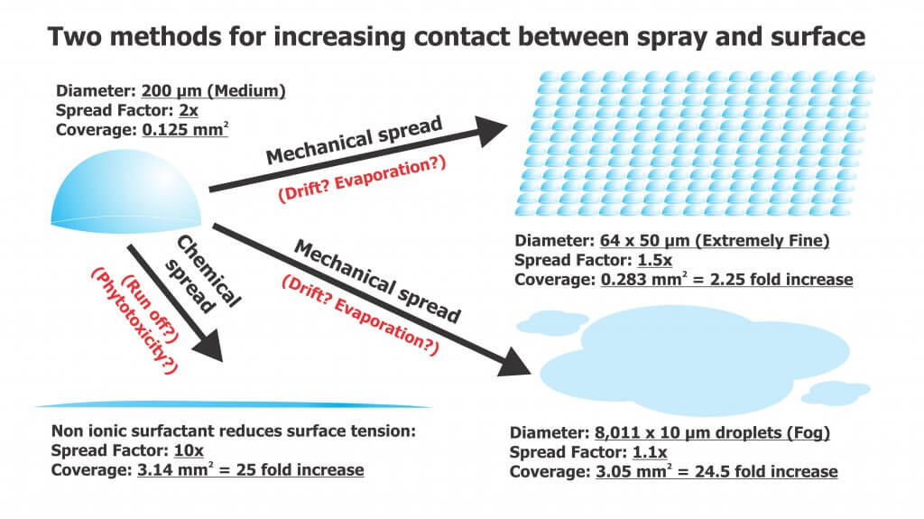
    Neither situation is desirable since the goal of spraying is to maximize the level of contact between droplet and target. Contact can be increased via mechanical spread or chemical spread (see figure below).

    The degree of chemical spread can be increased by adding adjuvants such as non-ionic surfactants to reduce surface tension. In the videos below we see the same controlled droplets with the same volume of liquid, but they now include a non-ionic surfactant. In the first video we see a greater degree of contact with the waxy target surface as the droplet spreads. In the second, the droplet does not get caught by the trichome, but splashes down onto the surface. Some product labels advise the inclusion of adjuvants and others are already formulated with them. In the case of surfactants, be aware of the potential for run-off and phytotoxicity.

    Mechanical spread requires us to break a single, larger droplet into several smaller volumes to increase the degree of contact. This approach usually comes with a caveat about evaporation, but this is rarely a concern in a humid greenhouse. As for the risk of drift, once again, in greenhouses it is a different story than conventional spraying. Spray drift is desirable! Lateral air movement is very important to encourage plant canopy penetration and prevent droplets from merely settling on upward-facing plant surfaces. While some equipment generates its own air, the air currents in the greenhouse are often the primary means for suspended droplets to circulate throughout the space. In either case, air could be considered the carrier instead of water. Too little air flow, or gaps in circulation, will reduce coverage. Too much air flow (specifically, greenhouse air circulation) may cause plants to exhibit stunting.

    Spray Quality (ISO)

    Here’s how ISO/DIS (5681:2019 Equipment for crop protection — Vocabulary 3.2.1) defines the spray quality produced by misters and foggers:

    • (3.2.1.13) MIST: “Spray with volume median diameter between 50 µm and 100 µm.”
    • (3.2.1.14) FOG: “Aerosol spray with volume median diameter under 50 µm where the droplets are effectively suspended in air with little or no settling by gravity.”

    These droplets do not behave like coarser droplets. For more information on droplet movement, survivability, and transfer efficiency, download Purdue Extension’s “Adjuvants and the Power of the Spray Droplet”.

    Water sensitive paper has limited utility when diagnosing coverage from foggers. Sophisticated optical scanners may be able to detect deposits as small as 25 µm, but this is open to debate. Manufacturers do not support the use of papers when quantifying deposits less than 50 µm , and some draw the line at 100 µm.

    In the following image, papers were used to diagnose coverage (from clean water) in a poinsettia greenhouse. The two papers on the right were located in the canopy and sprayed using a thermal pulse fogger and a hardware store style hand pump. The paper on the left was held directly in the path of the fogger while using the smallest nozzle provided with the unit. The spray enveloped the paper (and the person holding it). Close inspection showed tiny deposits, and the SnapCard app detected 4.5% coverage, but this greatly underestimates the actual deposition and does not account for the droplet count.

    UV dyes are the preferred method for analyzing coverage from foggers.

    Fogging and Misting Equipment

    Greenhouse spray equipment can be classified by droplet size, but also by the spray volume they employ.

    High Volume (HV)

    These applications are performed at pressures ranging from 500 to 4,285 kPa (75 to 700 psi) employing flow rates of 3.9 to 5.7 L/min (1 to 1.5 US g/min). They use standard label rates to accomplish a dilute application by broadcasting droplets larger than 100 microns. The goal is to cover all surfaces without incurring run-off. Examples of HV application equipment include backpack sprayers, trailed sprayers and boom sprayers. Practice and self-calibration are necessary to achieve the desired results when using manual HV sprayers.

    Targeted Low Volume (LV)

    These applications are performed at high pressures around 20,685 kPa (3,000 psi) employing flow rates approaching 1 L/min (0.26 US g/min), covering 93 m2 (1,000 ft2). They apply reduced rates over a given area and create droplets between 25 and 100 µm. These are concentrated sprays that do not result in wet foliage. LV applications are particularly good in high-humidity environments, when it is desirable to minimize the moisture on leaves. Examples of LV application equipment include aerosol cans.

    Ultra-Low Volume (ULV)

    These applications employ flow rates approaching 2 L/min (0.52 US g/min), covering 930 m2 (10,000 ft2). They require concentrated solutions, but apply reduced rates per area using droplets less than 25 µm. ULV applications will not raise greenhouse humidity and are a good choice when days are short and nights are long. They are also an excellent way to apply disinfectants for complete space sanitation before starting a new crop. It is important to ensure vents are closed and fans are off during sanitation. Examples of ULV application equipment include total release cans, auto foggers and thermal pulse foggers.

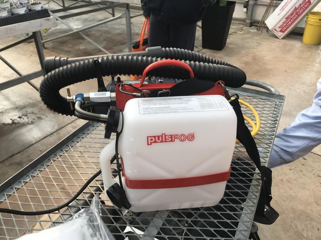
    PulsFOG hand-held ULV cold fogger

    Thermal pulse foggers are unlike other ULV equipment and warrant special consideration. The design of the pulse fogger has remained virtually unchanged since the 1940’s. Smaller, 24 hp machines are used in smaller operations but range up to large 175 hp machines. Tank size ranges from 10 to 50 L, where 10 L should be enough to cover 4,645 m2 (50,000 ft2) in about 10 minutes, depending on crop density. Their range is about 35 m (115 ft) from the point of release.

    Thermal Pulse foggers do not create aerosol using air shear – they use combustion (80 to 100 explosions per second) to shatter spray into a fog and propel it via positive pressure. Heat is a by-product of the engine, making it an unsuitable method for applying biological products.

    However, water-cooled foggers such as Dramm’s Bio Pulse Fogger reduce the exhaust temperature below 100 °C to make the application bio-rational. This has the added advantage of making droplet sizes more consistent and preventing spray from evaporating too quickly before it diffuses to the target.

    Dramm Bio Pulse Fogger.
    Dramm Bio Pulse Fogger

    Using a Fogger

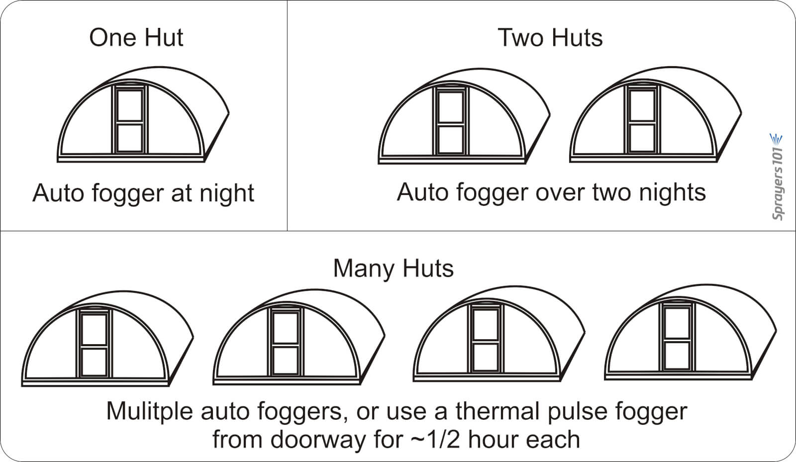
    Dramm recommends that operators use approximately 1 L of carrier in 5 L of spray mix, but a higher proportion of carrier would be required for more viscous products. Start with a full tank of clean, high grade gasoline and once the fogger has been started, run it continuously until the application is complete. Leave it running even when moving between Quonset huts (see below).

    Know when to use a pulse fogger versus an auto fogger. Auto foggers are convenient because the operator can set them and leave. However, in the case of multiple huts, it is more efficient and timely to use a thermal pulse fogger.
    Know when to use a pulse fogger versus an auto fogger. Auto foggers are convenient because the operator can set them and leave. However, in the case of multiple huts, it is more efficient and timely to use a thermal pulse fogger.

    Do not leave the manual fogger running unsupervised as an auto fogger: If they stay stationary, or aim directly at the canopy (as in hydraulic spraying), they could drench and potentially damage nearby plants.

    When fogging, aim between the plants, such as the alleys and between hanging plants. This allows the fog to expand and permeate canopies for the best coverage. When spraying is done, be sure to release the pressure created in the spray tank to prevent accidental back flow into the gasoline tank.

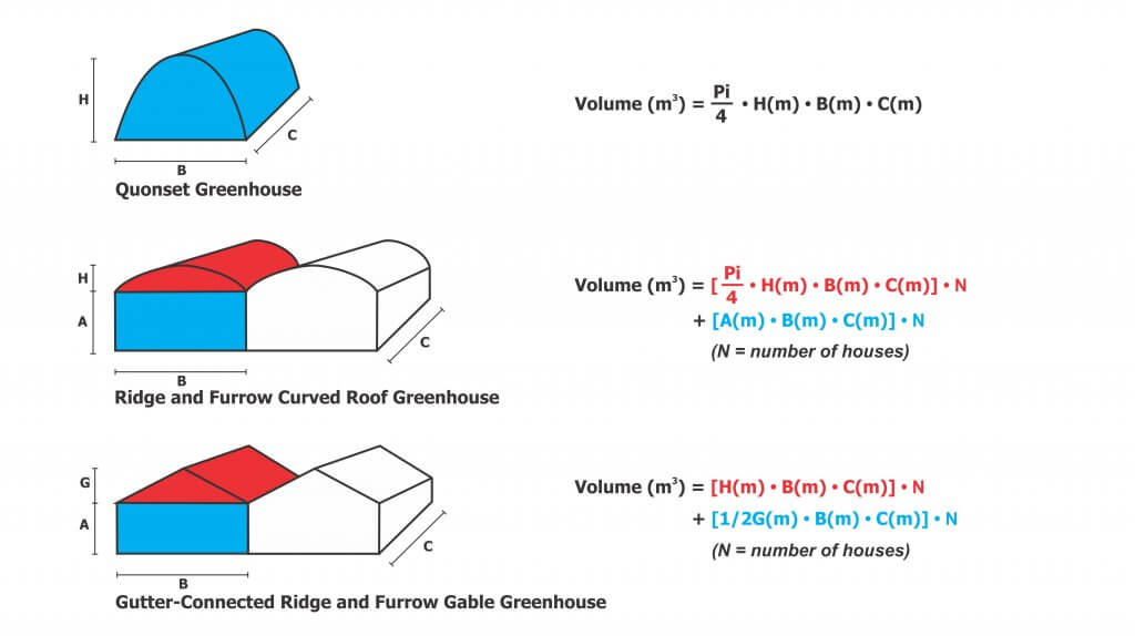
    And, because it’s convenient to include the math in this article, here are the formulae for calculating greenhouse volume to help you determine rates.

    Care and Maintenance

    HV, LV and ULV equipment requires model-specific cleaning and maintenance, according to manufacturer’s instructions. Even when sprayers are kept in prime condition, they are only as good as the operator’s understanding. When the wrong product is applied by the wrong machine using the wrong method, operators risk poor control, crop damage and increased potential for pesticide resistance. For more information, read the instructions that came with your sprayer, or contact the manufacturer.

    Thanks to Louis Damm and Dr. Heping Zhu for their contributions to this article.

    Try our calibration calculator:

  • Sprayer Math for Banded Applications

    Sprayer Math for Banded Applications

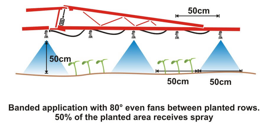
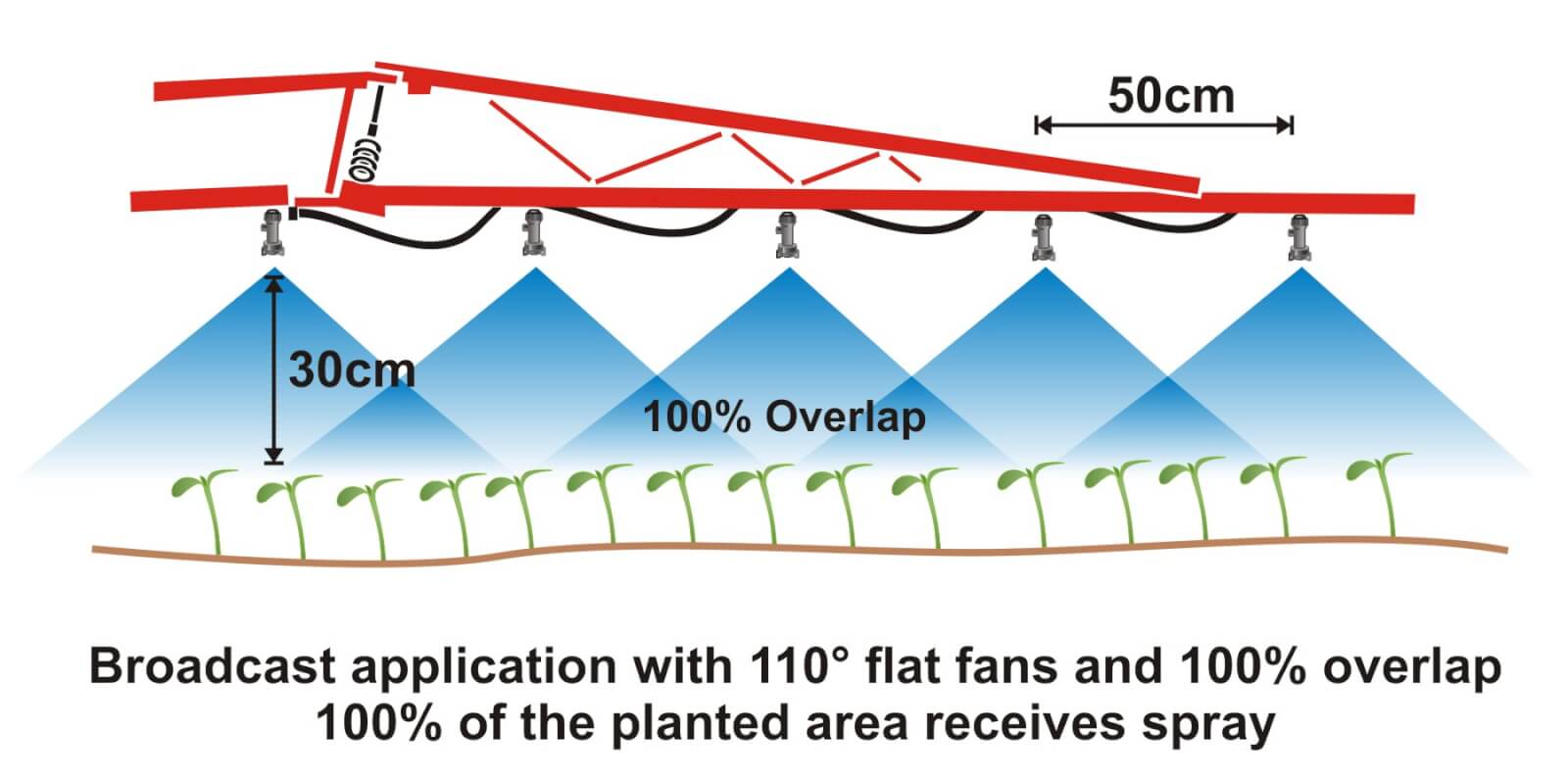
    Where crops are planted in rows, growers can save on chemical costs and reduce potentially wasted spray by performing banded applications. A banded application is treating parallel bands (Figure one), unlike a broadcast application where the entire area is treated (Figure two). This means only a portion of the field or orchard/vineyard floor receives spray, so the total amount of product applied per hectare (or per acre) should be less for banded than for broadcast.

    Figure 1
    Figure 1
    Figure 2
    Figure 2

    Banded applications are used in many situations, including:

    • Applying herbicides right over a crop during planting, both for pre-emergent or post-emergent crops.
    • Applying insecticides/fungicides by “directed spraying” using drop hoses or row kits; the latter is pictured in Figure three.
    • Carefully spraying herbicide between the rows to control weeds in the alleys of an established crop (Figure one).
    • Applying herbicide under fruit trees or grape vines to control weeds (Figure four).
    Figure 3
    Figure 3
    Figure 4
    Figure 4

    It’s easy to make mistakes when calculating product rates for banded applications and these can be costly errors: too little means poor control and too much means wasted product and possible crop injury. This article describes how to calculate sprayer output and product rate for common banded applications.

    Step One: Determine broadcast volume

    Pesticide labels typically list broadcast product rates (e.g. amount of formulated product per hectare or acre). In this example, let’s say the label recommends a broadcast product rate of 500 ml of formulated herbicide applied using 100 litres of spray mix per hectare (i.e. added to 99.5 L water).

    Step Two: Establish sprayer settings

    Select a travel speed that is safe, gives decent efficiency and doesn’t compromise coverage. For this example, we’ll say the sprayer moving is at 8.0 km/h.

    Select a band width that completely covers the target row and some of the adjacent area where control is desired. Band width should be measured along the ground for soil-applied products or along the top of plants for post-emergence products. We’ll use Figure one for our settings: bands are 50 cm wide on 100 cm centres. We’ll say that a single nozzle swath can treat the band, and that we’re spraying 2 hectares of planted area.

    Step Three: Calculate the banded sprayer output

    We can calculate how much of the planted area actually receives spray using this formula:

    [band width (cm) ÷ row width (cm)] x total planted area (ha) = actual sprayed area (ha)
    [50 cm ÷ 100 cm] x 2 ha = 1 ha

    For completeness, here’s the US formula:
    [band width (in) ÷ row width (in)] x total planted area (ac) = actual sprayed area (ac)

    From this we now know that we should be able to go twice as far on a tank spraying a banded application as we would a broadcast, because we’re only spraying half the planted area.

    Step four: Calculate the nozzle output

    Use the following formula to convert the broadcast output into the banded output:

    [broadcast output (L/ha) x travel speed (km/h) x (swath width (cm) ÷ number of nozzles per swath)] ÷ 60,000 = nozzle output (L/min)
    [100 L/ha x 8 km/h x (50 ÷ 1)] ÷ 60,000 = 0.67 L/min

    For completeness, here’s the US formula:
    [broadcast output (gal/ac) x travel speed (mph) x (swath width (in) ÷ number of nozzles per swath)] ÷ 5,940 = nozzle output (gal/min)

    If multiple nozzles were contributing to the swath, such as in figure three or figure four, this formula will account for it. You still mix the labelled product rate at a ratio of 500 ml of herbicide to 99.5 L water, but as we determined in step three, we should be able to spray twice the planted area using a banded application as we would a broadcast application.

    Warning! Watch your units. You may be familiar with other formulae for calculating your output. Do not mix and match formulae or parts of formulae. For example, here is another Metric option for determining L/min. It employs different units so it requires a different constant:

    [broadcast output (L/ha) x travel speed (m/min) x (swath width (m)) ÷ number of nozzles per swath)] ÷ 10,000 (m2/ha) = nozzle output (L/min)

    Step Five: Use the nozzle catalogue to find the right nozzle

    Using a nozzle manufacturer’s catalogue, select a nozzle that gives the desired spray quality (usually coarser for herbicides) and will produce the 50 cm swath we’re looking for (which can be adjusted a little using boom height). Always choose to operate a nozzle in the middle of its pressure range.

    Step Six: Calibrate the sprayer (i.e. double-check)

    Follow your typical calibration process and make minor adjustments until the nozzle discharge per minute results in the desired banded output. A rate controller will handle this on larger sprayers, but if you don’t have one you can make small adjustments to speed and pressure until the desired output is achieved. Ideally, if your math was right, these changes won’t be needed.

    When performed correctly, banded applications are a great way to focus your efforts on the target, saving time and money.

    Other Resources

    Download this booklet on spraying potatoes using banded rows. Or try our calculator:

  • OrchardMAX 2.0

    OrchardMAX 2.0

    2016_Orchard_Max_Logo

    OrchardMAX won the 2016 Canadian Agri-Marketing Association’s “Certificate of Merit” in the Mobile Apps Category.

    OrchardMAX is a free decision-support tool that helps apple growers match airblast sprayer output to the size, shape, and density of an orchard canopy.

    Rather than applying the same volume and pesticide dose to every block throughout the season, OrchardMAX uses the principles of Crop-Adapted Spraying to estimate settings appropriate for each orchard block. The objective is more consistent spray coverage with less avoidable waste. Ontario and Nova Scotia orchard trials demonstrated seasonal spray-volume savings of approximately 20 to 35%, without significant differences in pest activity and reported or fruit quality.

    What OrchardMAX does

    Using information supplied by the operator, OrchardMAX can:

    • Account for changes in canopy size, shape, and density
    • Estimate an appropriate carrier volume and pesticide dose
    • Suggest nozzle flow rates and sprayer settings
    • Calculate the amount of formulated product required per tank
    • Estimate work rate, tank requirements, and potential savings

    What OrchardMAX does not do

    OrchardMAX is a decision-support tool, not a substitute for calibration, operator judgement, or the pesticide label. It will not:

    • Recommend a rate above the pesticide label
    • Calibrate the sprayer
    • Confirm that adequate spray coverage was achieved
    • Account fully for wind, temperature, or relative humidity
    • Recommend less than 400 L/ha, approximately 42.5 US gal/ac
    • Recommend less than half the labelled pesticide rate

    The results are only as reliable as the information entered. Operators must still maintain and calibrate the sprayer, match air settings to the canopy, work in reasonable weather conditions and confirm coverage using water-sensitive paper.

    How to use it

    For each spray scenario:

    • Select or enter the sprayer and orchard block.
    • Describe the current canopy size, shape, and density.
    • Enter the labelled pesticide rate and planned spray mixture.
    • Review the proposed carrier volume, pesticide dose, nozzle rates, and number of tanks.
    • Configure and calibrate the sprayer.
    • Confirm the resulting coverage in the orchard and adjust where necessary.

    Start with a few representative blocks. Compare OrchardMAX recommendations with your current program, evaluate coverage, and make incremental changes as you gain confidence.

    History

    The original app was an excel-based tool created in 2010 and later developed into an app for iOS and Android systems by AgNition Inc. with funding from Growing Forward 2 in 2016. Compatibility with iOS and Android ended in 2020. We have now rebuilt the same functionality into this online version of the app.

  • What is Spray Quality, Part 4 – An Important Change in S572.3 and ISO25358

    What is Spray Quality, Part 4 – An Important Change in S572.3 and ISO25358

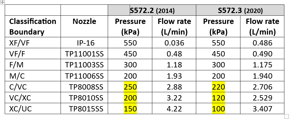
    A new version of standard ASABE S572.3 (adopted 2020) and its international equivalent, ISO 25358 (adopted 2018) addresses a limitation of the previous standards. In ASABE S572.2, the nozzle that defined the category boundary between the XC and UC sprays was the TP8015 SS at 4.22 L/min, corresponding to 150 kPa. Only very few nozzles produced UC sprays, and those that did only did so at the lower pressures and higher flow rates. For those nozzles, the categories worked.

    The emergence of a host of new low-drift nozzles designed to meet the regulatory requirement for drift protection for Xtendimax and other dicamba formulations in soybeans revealed the limitation of this boundary nozzle choice. In essence, all the new dicamba-compliant low drift sprays were UC, regardless of nominal flow rate or spray pressure. Any effect of, say, higher pressure that would create a finer spray, was not revealed. It was decided that new boundary nozzles were needed so that the coarser sprays’ response to flow rate, pressure, and formulation or adjuvant choice, could be better described.

    S572.3 therefore lowered the defining flow rate of the XC/UC nozzle from 4.22 to 3.41 L/min, with a new spray pressure of 100 kPa (from 150 kPa). This made the new boundary spray coarser. Because this change made the adjacent spray quality class, the XC, broader, the VC and C categories were each also widened somewhat, by lowering their respective boundary nozzle flow rates and pressures (Table 1).  

    Table 1: Change in spray pressure of three coarsest boundary nozzles from ASABE S572.2 to S572.3

    For XF, VF, F, and M spray classes, there is no change with this new standard because the boundary nozzle conditions were not changed. But the C, VC, XC, and UC classes became coarser.

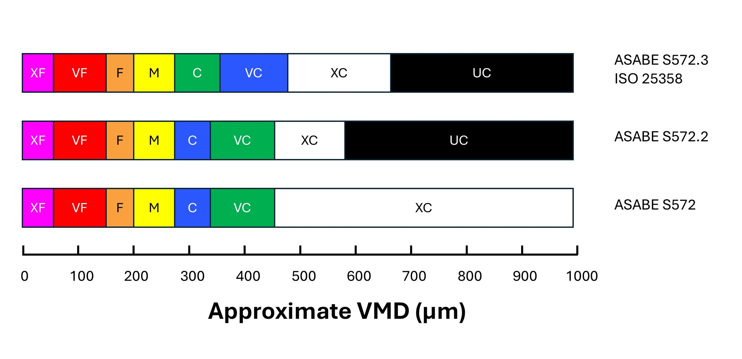
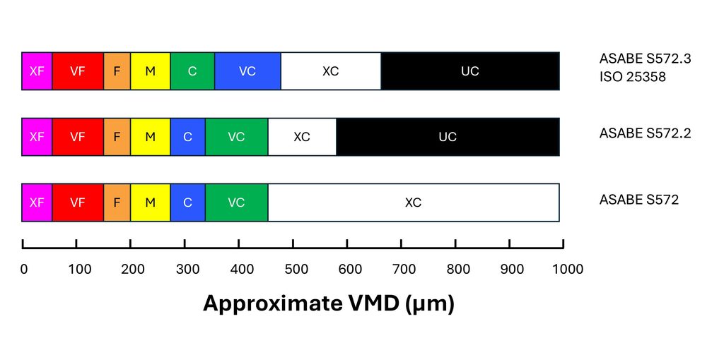
    In order to signal the change to consumers, the colour coding of the Coarse and Very Coarse sprays was switched. With S572.2, C was blue and VC was green. With S572.3, C is now green and VC is blue (Figure 1). 

    Figure 1: Approximate changes in the Volume Median Diameter (VMD) of boundary nozzles under the S572 standard versions. Note that the coarsest spray quality categories are more equally distributed in the newest standard versions.

    The change means that low-drift sprays categorized using S572.2 can no longer be accurately compared to nozzles categorized using S572.3. For example, if a researcher conducted efficacy studies and concluded that ASABE S572.2 Coarse sprays provided acceptable efficacy, but S572.2 Very Coarse sprays had lower performance, they might recommend Coarse sprays. But would that recommendation be safe for nozzles classified with S572.3? In that standard, the C category extends into the territory formerly occupied by VC, deemed too coarse by the research.

    A similar problem exists for spray drift risk assessments. Let’s say a regulator recommends a 25 m buffer zone for ASABE S572.2 VC sprays based on modelling the drift from that C/VC boundary nozzle. What will the buffer zone be for the new S572.3 VC spray? Since the newer VC spray is coarser at its lower boundary, drift, and therefore the buffer zone, would be less. Determining how much so would require a new spray drift dataset for the new boundary nozzle.

    In fairness, most of the risk assessments are done on finer sprays such as Medium and Coarse, and those would remain unchanged because to be conservative, the regulator would assume the finest spray within each category (i.e., the lower boundary nozzle). But when a registrant requests that risk assessment be done with a coarser spray quality such as VC, XC, or UC, the regulator would need a new dataset.

    Another problem is that not all spray quality data reported by manufacturers use the new standard. Of the major North American manufacturers, Spraying Systems started reporting their products using the S572.3 standard in 2023. Pentair Hypro, and by extension John Deere, as well as Wilger Industries have not yet followed suit.

    The European manufacturers are well on their way. Agrotop (Greenleaf in the US), Lechler and Arag are both reporting using ISO 25358. But Billericay Farm Systems (BFS) are still reporting using the older standard.

    It may have been some years since nozzle manufacturers last tested the spray quality of their nozzles. If they now measure their sprays using the new standard, some other changes have also have ocurred in the interim. For example, new laser measurement systems may have been acquired. New scanning techniques may have been developed. New staff are operating the systems. And while the ASABE and ISO reference nozzles are intended to negate these differences, we are still seeing some discrepancies. It is also possible that changes to the manufacturing of the nozzles has also altered the spray quality they produce.

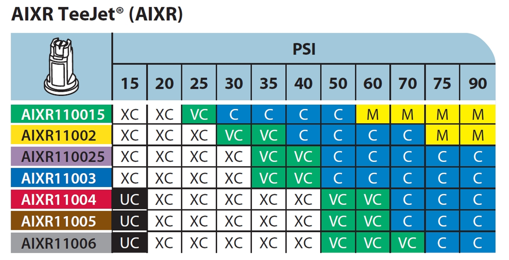
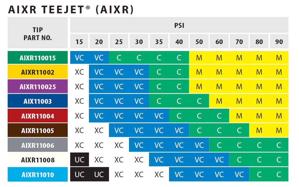
    For example, compare Figure 2, the TeeJet AIXR nozzle spray quality chart, developed using ASABE S572.2 and published in 2015, to Figure 3, the same nozzle whose spray quality was categorized using ASABE S572.3 and published in 2023.

    Figure 2: Spray quality of TeeJet AIXR tips according to S572.2, published by Spraying Systems in 2015. Reproduced from TeeJet Catalog 51A.

    First, let’s compare the portion of the chart that reports Medium spray qualities in Figure 2 to that in Figure 3. These should be the same given that the same boundary nozzle and pressure was used in both. But under the new testing, the region reporting a Medium spray has significantly expanded towards the lower pressures. The Medium sprays begin at 60 and 75 psi in the old standard, but at 50 psi for the new standard.

    Spray quality of TeeJet AIXR tips according to S572.3, published by Spraying Systems in 2023. Reproduced from TeeJet Catalog 52.

    The region occupied by the Coarse category has shifted towards lower pressures, as expected with the coarser upper (C/VC) boundary nozzle. It would be wider, as was the intent, had the M catergory not encroached.

    The region occupied by VC and XC have grown towards the lower left, more or less as expected. The VC category in particular, now dominates in the lower pressure region, a space previously occupied by the XC category. The small region which the UC category occupied under S572.2 in Figure 7 was replaced entirely by the XC category.

    Looking at it another way, the commonly used AIXR11004 size at pressures between 30 and 90 psi would have produced XC, VC, and C spray qualities in the old catalogue. The same nozzle now apparently produces VC, C, and M sprays at the same pressure range.

    These changes may or may not extend across all nozzles and manufacturers to the same extent as this example illustrates. But they add another level of complexity, and perhaps confusion, to applicators striving to be compliant with label directions. I am hopeful that the sector can quickly move to adopt the changes universally so that the mixed messaging is short lived and mistakes are minimized.  

    In particular, the regulatory bodies that rely on these spray quality classes to communicate drift potential and buffer zones must recognize that their risk assessments will need to reflect these new standards as more nozzle manufacturers begin communicating them.

    Droplet size continues to explain most of what matters in spraying, from deposition uniformity, to coverage and spray drift. Hopefully this series of articles explaining the measurement of spray droplet sizes is useful and sheds some light on how the industry measures and communicates it.