Category: Boom Sprayers

Main category for sprayers with horizontal booms

  • Spray Window – Can you plan a spray week?

    Spray Window – Can you plan a spray week?

    Plan the day. Weigh the risks. Finish the job.

    Spray Window is a strategy game about spray planning. You have one sprayer and six working days of changeable weather. Depending on your role, you manage your own fields or a list of clients’ jobs.

    Each turn is one day. Read the forecast and what each field needs, choose which jobs to do and in what order, set up the sprayer, and see how the day unfolds. There’s no single right answer.

    It’s what every operator learns on the job: assess the work, plan ahead, weigh risk against reward, and get as much done as you safely can. A week takes about 20 minutes and plays best on a tablet or computer. At the end, a debrief shows what your decisions cost, what they saved, and how a benchmark operator planned the same week.

    Why a game?

    Sprayer training usually covers drift, Delta T, inversions, spray quality, water volume, travel speed one at a time. On a real morning they all arrive together, along with crop stage, a closing window, a neighbour, and someone waiting on the work.

    Those decisions rarely have one correct answer, so they’re hard to teach in an article or test with a quiz. An owner facing a closing disease window might reasonably accept more drift risk than a custom applicator whose business depends on reputation. Both may be making a sound call.

    A simulation lets you decide, live with the consequences and try again. In Spray Window, the opponent is the weather and the clock, not another player. And, of course, it’s a fun 16-bit style that reminds me of a lot of wasted quarters in my youth.

    How it plays

    The game is set in Ontario mostly on corn, soybeans and winter wheat, with canola, white beans, sugar beets, processing tomatoes and potatoes in some weeks. Every week is a new combination of fields, crops, pests and weather, in one of three seasons.

    Choose your role (owner-operator or custom applicator) and your level, outfit your sprayer on a limited budget, pick your tires, and dive in. The weather changes, and there are surprises to deal with.

    There are three levels.

    • Beginner is a quiet week of seven fields: honest work orders, no surprises, no tank cleanouts and nobody pushing you to spray, and the sprayer comes ready to go.
    • Intermediate has ten fields and adds wind gusts, an interruption, wet ground, cleanouts and people leaning on you.
    • Expert is the full game. Your week is saved each morning, so you can stop and come back to it.

    Micron Woman is back to be your guide.

    Choose your role and level – the scenarios change accordingly.

    Spring

    In mid-May, jobs include herbicide and fungicide in wheat, a pre-emergence herbicide before the corn comes up, a burndown ahead of soybean planting, and insecticide for cereal leaf beetle and black cutworm at threshold.

    Early Summer

    In mid-June, jobs include fusarium head blight at wheat flowering, a Group 4 herbicide before the corn’s crop-stage limit, post-emergence herbicides in soybeans, and armyworm in wheat.

    Mid-Summer

    In late July, jobs include tar spot at corn tassel, white mould and soybean aphid in soybeans, western bean cutworm, and a pre-harvest herbicide as wheat dries down. 

    Drift

    Every field borders something sensitive: open water, a neighbour’s home and garden, beehives in a flowering hedgerow, a vineyard or a certified organic farm. Each responds as it would in real life.

    When water or habitat is downwind, the label may require an unsprayed buffer, and coarser sprays shrink it. Coarser sprays also cut drift sharply, because each step coarser roughly halves the fine droplets that drift, but fungicides and insecticides lose some coverage, so more water helps them. Heat brings another risk: after application, dicamba can turn to vapour and move off target whatever the nozzle. In June, a cooler day or a pass after the heat of the day may be the safer call.

    Sometimes, not spraying is the right move.

    Outfit your sprayer for the week ahead.

    High scores, weekly scenarios and feedback

    Money keeps score. Beside your money, a second readout shows whether you’re ahead (▲) or behind (▼) the benchmark operator playing the same week. Every off-label pass is a label strike and a fine, so bad calls sting right away. If your balance falls below zero, you’re broke and the week ends with zero points.

    A score of 1,000 means you finished as well off as the benchmark. Both roles use the same yardstick, and weeks are drawn from scenarios of similar difficulty, so scores are comparable. Each level has its own benchmark and its own high scores, so beginners compete with beginners.

    Ranks are awarded as follows: 

    • Apprentice (0-499)
    • Operator (500+)
    • Pro (800+)
    • Ace (950+)
    • Legend (1,100+)
    Get your rank and scorecard. See what you might have done differently.

    At the end of the week you get your report card. “Turning points” shows the three decisions that cost you most and what the forecast would have allowed instead. If you want to understand how the game balances all these variables, check out the (assumptions) button.

    Enter your initials arcade-style. Your score is sent to the leaderboard automatically and once we review it, the leaderboard updates. Playing a downloaded copy? Email the code from the end screen to jason@sprayers101.com. Something odd, or a call you’d question? Copy the code and send it with a note: your exact week can be replayed. Only a week’s first play counts; “Play this week again” is for practice.

    Thanks to Dr. Ian McDonald for the inspiration to build a game. Ready to play?

    High Scores

    1. 1RKLegendCustom applicator1,102points
    2. 2JAYAceOwner-operator1,072points
    3. 3RKAceCustom applicator994points

    See the full leaderboard

    Version Updates:

    Updated November 6, 2026: Three levels, Beginner, Intermediate and Expert, each with its own high scores. A week in progress is saved on your device, so you can finish it later. And on still mornings, listen for a train in the distance. Scores from earlier versions count as Expert.

    Updated November 5, 2026: Refills and water volume now add up correctly, so more water never makes a job finish sooner (thanks, Lucas). Each job card now shows how the product moves, its Group and its rainfast time, and the day plan warns when rain could wash it off. Micron Woman’s tutorial is clearer and shorter. Scores from earlier versions still count.

    Updated November 2, 2026: Spray quality and walking the edges rebalanced so careful decisions pay off more, and the top three scores now appear on the title screen between rounds. Scores from earlier versions still count.
  • How Much Pesticide in the Tank?

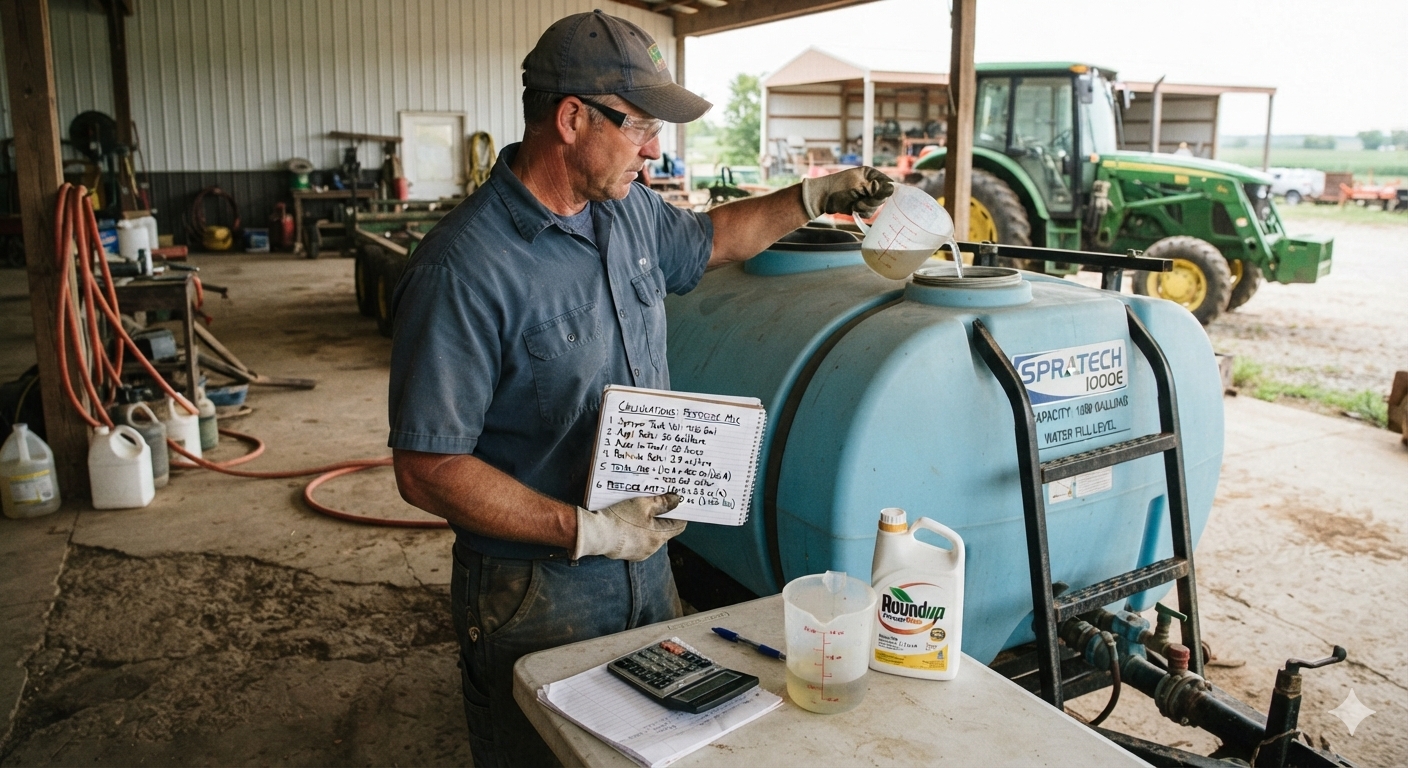
    How Much Pesticide in the Tank?

    Sprayer math can be intimidating, but the effort gives solid value. When combined with a calibrated sprayer you reap the following benefits:

    • Determine how much spray mix is required to apply the intended rate.
    • Estimate how much crop protection product must be ordered for the season.
    • Populate spray records which allow you to review practices, respond to enquiries and satisfy traceability requirements.

    There are many ways to perform sprayer math, and you need only look to local pesticide safety courses, industrial catalogues, and extension resource centres for examples. If you’re already comfortable with your current method, don’t mix and match with others. Sprayer math is a series of related calculations that employ constants to keep the units straight. It’s all or none.

    Walkthrough

    Let’s start with the classic, US Imperial formula for calculating the sprayer output. We’ll weave in Metric, later. This base formula can be adjusted to allow you to solve for any factor, as long as you’re only missing one piece of information. Turns out your high school teacher was right – you DO need algebra.

    GPM = [GPA x MPH x W] ÷ 5,940

    In this case, you can determine an output rate (GPM – gallons per minute). You’ll need to know your target volume (GPA – gallons per acre), your average travel speed (MPH – miles per hour) and your nozzle spacing (W – which is width in inches). The number “5,940” is a constant that handles all the unit conversions. If you divide the GPM by the number of nozzles on your sprayer (assuming they are all the same rate), you can hone in on the ideal nozzle size.

    But, as we noted earlier, you can do a lot more with sprayer math than just pick the ideal nozzle size. The rest of this article includes examples of both Metric and US Imperial formulae, but watch out for unit conversions. If at any time you don’t see the units you’re looking for, you can consult our unit conversion tool.

    Grab your calculator – it’s math time!

    Don’t be intimidated. With a little practice, sprayer math gets easier and it’s always worthwhile. The real trick is navigating unit conversions.

    Step 1 – How large is the area you need to spray?

    Multiply the length of the area you plan to spray times the width. If you are using metres, then divide the product by 10,000, which is the number of m2 in a hectare (ha). For feet and acres, divide by 43,560 which is the number of ft2 in an acre (ac):

    Step 2 – How much product is needed to spray the area?

    Consult the rate(s) shown on the label. In Canada, rates are often based on planted area (E.g. hectares). In Australia and New Zealand, they may be based on row length (not covered in this article). If you measure your area in acres, you’ll have to convert the rate by multiplying by a constant: 0.4.

    product-per-area

    Now multiply the area you want to spray (step 1) by the rate (step 2).

    product-per-area2

    Step 3 – How far can you go on a full tank?

    You know your sprayer output (determined through calibration) so you divide that into your tank size. Watch your units:

    full-tank-distance

    Step 4 – How much pesticide per tank? 

    Multiply the area that can be sprayed per tank (Step 3) by the pesticide rate (Step 2). Again, watch your units:

    pesticide-per-tank

    Step 5 – How much area is left to spray?

    Just subtract what you’ve already sprayed from the total area.

    area-left-to-spray

    Step 6 – How much pesticide in the last, partially-full tank?

    Multiply the area you have left to spray (Step 5) by the pesticide rate (Step 2). Yes, watch your units:

    pesticide-partially-full-tank

    Step 7 – How much spray mix will I need for the partial tank to finish spraying the total area?

    Multiply the area you have left to spray (Step 5) by the sprayer output (determined through calibration). Guess what? Watch your units:

    spray-mix-for-total-area

    Sample problems

    Time to test your knowledge. Let’s suppose you want to apply a product rate of 3 L/ha to your blueberries. You calibrate your sprayer and determine your output to be 50 L/ha. Your tank holds 400 L of spray mix. Your planting is 500 m long and 200 m wide.

    Q1 – How large is the area you need to spray?

    area-to-spray

    Q2 – How much product is needed to spray the area?

    product-to-spray-the-area

    Q3- How much area can be sprayed on one tank?

    area-on-full-tank

    Q4 – How much product should be added to a full tank?

    product-needed-full-tank

    Q5 – After the tank is empty, how much area is left to spray?

    area-left

    Q6 – How much product to add to the last, partially full tank?

    product-partially-full-tank

    Q7 – How much spray mix will be needed to finish spraying?

    spray-mix-to-finish-spraying

    Tank mix calculator

    You might feel we buried the lead by adding this calculator to the end of the article. It’s important for a sprayer operator to understand the math required to interpret labels and calculate tank mixes, so hopefully you read and understood the process before you got here. And now that you have, this is a very helpful tool. Try it online, or download a standalone version.

    Notable exceptions

    Certain situations aren’t covered in this article. If you are spraying a greenhouse, the math is different. If you are performing a banded application, the math is different. And, if you’re an airblast operator trying to reconcile why a pesticide label uses planted area rather than canopy volume for its rates, you’re in for some additional reading.

  • Sprayer Math for Banded Applications

    Sprayer Math for Banded Applications

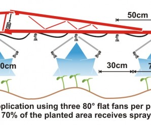
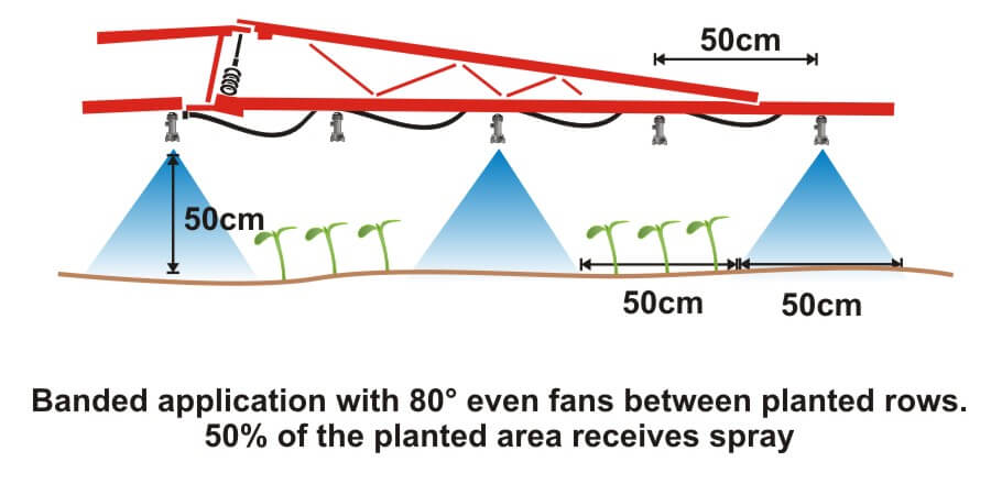
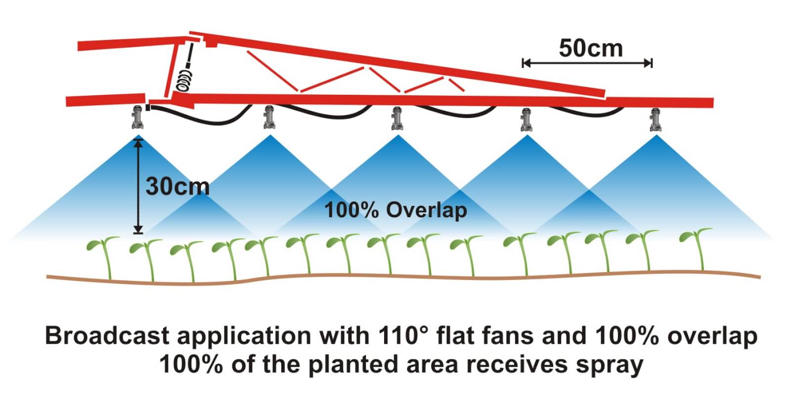
    Where crops are planted in rows, growers can save on chemical costs and reduce potentially wasted spray by performing banded applications. A banded application is treating parallel bands (Figure one), unlike a broadcast application where the entire area is treated (Figure two). This means only a portion of the field or orchard/vineyard floor receives spray, so the total amount of product applied per hectare (or per acre) should be less for banded than for broadcast.

    Figure 1
    Figure 1
    Figure 2
    Figure 2

    Banded applications are used in many situations, including:

    • Applying herbicides right over a crop during planting, both for pre-emergent or post-emergent crops.
    • Applying insecticides/fungicides by “directed spraying” using drop hoses or row kits; the latter is pictured in Figure three.
    • Carefully spraying herbicide between the rows to control weeds in the alleys of an established crop (Figure one).
    • Applying herbicide under fruit trees or grape vines to control weeds (Figure four).
    Figure 3
    Figure 3
    Figure 4
    Figure 4

    It’s easy to make mistakes when calculating product rates for banded applications and these can be costly errors: too little means poor control and too much means wasted product and possible crop injury. This article describes how to calculate sprayer output and product rate for common banded applications.

    Step One: Determine broadcast volume

    Pesticide labels typically list broadcast product rates (e.g. amount of formulated product per hectare or acre). In this example, let’s say the label recommends a broadcast product rate of 500 ml of formulated herbicide applied using 100 litres of spray mix per hectare (i.e. added to 99.5 L water).

    Step Two: Establish sprayer settings

    Select a travel speed that is safe, gives decent efficiency and doesn’t compromise coverage. For this example, we’ll say the sprayer moving is at 8.0 km/h.

    Select a band width that completely covers the target row and some of the adjacent area where control is desired. Band width should be measured along the ground for soil-applied products or along the top of plants for post-emergence products. We’ll use Figure one for our settings: bands are 50 cm wide on 100 cm centres. We’ll say that a single nozzle swath can treat the band, and that we’re spraying 2 hectares of planted area.

    Step Three: Calculate the banded sprayer output

    We can calculate how much of the planted area actually receives spray using this formula:

    [band width (cm) ÷ row width (cm)] x total planted area (ha) = actual sprayed area (ha)
    [50 cm ÷ 100 cm] x 2 ha = 1 ha

    For completeness, here’s the US formula:
    [band width (in) ÷ row width (in)] x total planted area (ac) = actual sprayed area (ac)

    From this we now know that we should be able to go twice as far on a tank spraying a banded application as we would a broadcast, because we’re only spraying half the planted area.

    Step four: Calculate the nozzle output

    Use the following formula to convert the broadcast output into the banded output:

    [broadcast output (L/ha) x travel speed (km/h) x (swath width (cm) ÷ number of nozzles per swath)] ÷ 60,000 = nozzle output (L/min)
    [100 L/ha x 8 km/h x (50 ÷ 1)] ÷ 60,000 = 0.67 L/min

    For completeness, here’s the US formula:
    [broadcast output (gal/ac) x travel speed (mph) x (swath width (in) ÷ number of nozzles per swath)] ÷ 5,940 = nozzle output (gal/min)

    If multiple nozzles were contributing to the swath, such as in figure three or figure four, this formula will account for it. You still mix the labelled product rate at a ratio of 500 ml of herbicide to 99.5 L water, but as we determined in step three, we should be able to spray twice the planted area using a banded application as we would a broadcast application.

    Warning! Watch your units. You may be familiar with other formulae for calculating your output. Do not mix and match formulae or parts of formulae. For example, here is another Metric option for determining L/min. It employs different units so it requires a different constant:

    [broadcast output (L/ha) x travel speed (m/min) x (swath width (m)) ÷ number of nozzles per swath)] ÷ 10,000 (m2/ha) = nozzle output (L/min)

    Step Five: Use the nozzle catalogue to find the right nozzle

    Using a nozzle manufacturer’s catalogue, select a nozzle that gives the desired spray quality (usually coarser for herbicides) and will produce the 50 cm swath we’re looking for (which can be adjusted a little using boom height). Always choose to operate a nozzle in the middle of its pressure range.

    Step Six: Calibrate the sprayer (i.e. double-check)

    Follow your typical calibration process and make minor adjustments until the nozzle discharge per minute results in the desired banded output. A rate controller will handle this on larger sprayers, but if you don’t have one you can make small adjustments to speed and pressure until the desired output is achieved. Ideally, if your math was right, these changes won’t be needed.

    When performed correctly, banded applications are a great way to focus your efforts on the target, saving time and money.

    Other Resources

    Download this booklet on spraying potatoes using banded rows. Or try our calculator:

  • What is Spray Quality, Part 4 – An Important Change in S572.3 and ISO25358

    What is Spray Quality, Part 4 – An Important Change in S572.3 and ISO25358

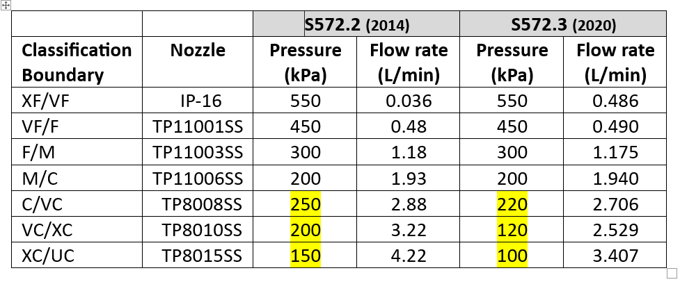
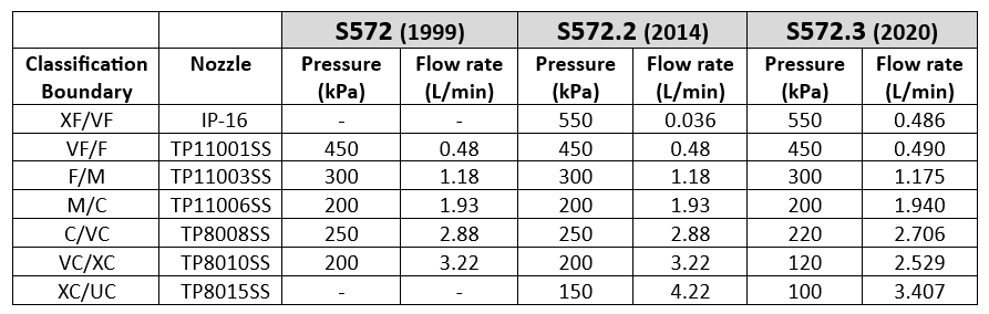
    A new version of standard ASABE S572.3 (adopted 2020) and its international equivalent, ISO 25358 (adopted 2018) addresses a limitation of the previous standards. In ASABE S572.2, the nozzle that defined the category boundary between the XC and UC sprays was the TP8015 SS at 4.22 L/min, corresponding to 150 kPa. Only very few nozzles produced UC sprays, and those that did only did so at the lower pressures and higher flow rates. For those nozzles, the categories worked.

    The emergence of a host of new low-drift nozzles designed to meet the regulatory requirement for drift protection for Xtendimax and other dicamba formulations in soybeans revealed the limitation of this boundary nozzle choice. In essence, all the new dicamba-compliant low drift sprays were UC, regardless of nominal flow rate or spray pressure. Any effect of, say, higher pressure that would create a finer spray, was not revealed. It was decided that new boundary nozzles were needed so that the coarser sprays’ response to flow rate, pressure, and formulation or adjuvant choice, could be better described.

    S572.3 therefore lowered the defining flow rate of the XC/UC nozzle from 4.22 to 3.41 L/min, with a new spray pressure of 100 kPa (from 150 kPa). This made the new boundary spray coarser. Because this change made the adjacent spray quality class, the XC, broader, the VC and C categories were each also widened somewhat, by lowering their respective boundary nozzle flow rates and pressures (Table 1).  

    Table 1: Change in spray pressure of three coarsest boundary nozzles from ASABE S572.2 to S572.3

    For XF, VF, F, and M spray classes, there is no change with this new standard because the boundary nozzle conditions were not changed. But the C, VC, XC, and UC classes became coarser.

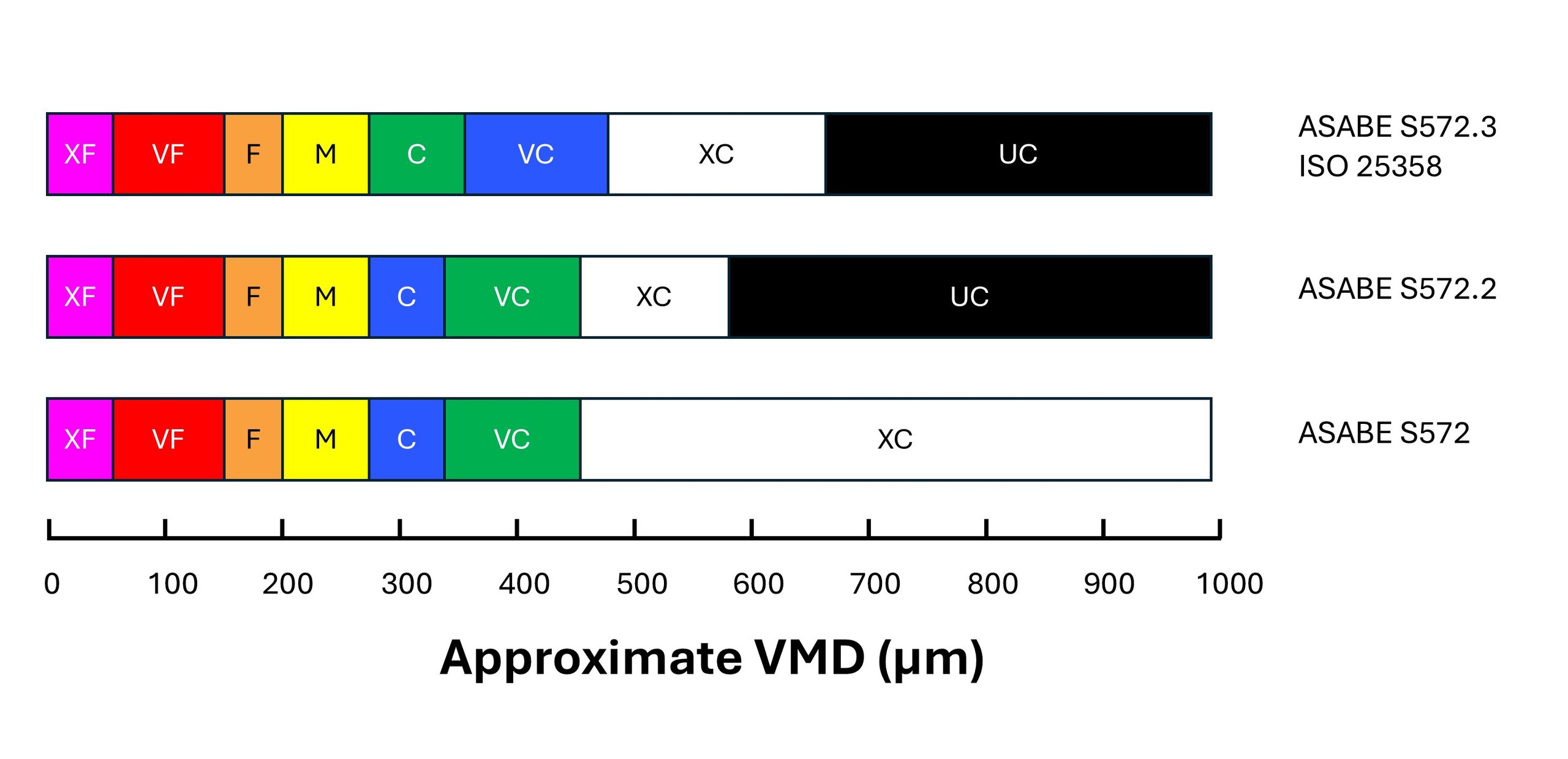
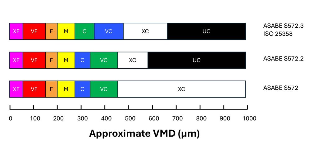
    In order to signal the change to consumers, the colour coding of the Coarse and Very Coarse sprays was switched. With S572.2, C was blue and VC was green. With S572.3, C is now green and VC is blue (Figure 1). 

    Figure 1: Approximate changes in the Volume Median Diameter (VMD) of boundary nozzles under the S572 standard versions. Note that the coarsest spray quality categories are more equally distributed in the newest standard versions.

    The change means that low-drift sprays categorized using S572.2 can no longer be accurately compared to nozzles categorized using S572.3. For example, if a researcher conducted efficacy studies and concluded that ASABE S572.2 Coarse sprays provided acceptable efficacy, but S572.2 Very Coarse sprays had lower performance, they might recommend Coarse sprays. But would that recommendation be safe for nozzles classified with S572.3? In that standard, the C category extends into the territory formerly occupied by VC, deemed too coarse by the research.

    A similar problem exists for spray drift risk assessments. Let’s say a regulator recommends a 25 m buffer zone for ASABE S572.2 VC sprays based on modelling the drift from that C/VC boundary nozzle. What will the buffer zone be for the new S572.3 VC spray? Since the newer VC spray is coarser at its lower boundary, drift, and therefore the buffer zone, would be less. Determining how much so would require a new spray drift dataset for the new boundary nozzle.

    In fairness, most of the risk assessments are done on finer sprays such as Medium and Coarse, and those would remain unchanged because to be conservative, the regulator would assume the finest spray within each category (i.e., the lower boundary nozzle). But when a registrant requests that risk assessment be done with a coarser spray quality such as VC, XC, or UC, the regulator would need a new dataset.

    Another problem is that not all spray quality data reported by manufacturers use the new standard. Of the major North American manufacturers, Spraying Systems started reporting their products using the S572.3 standard in 2023. Pentair Hypro, and by extension John Deere, as well as Wilger Industries have not yet followed suit.

    The European manufacturers are well on their way. Agrotop (Greenleaf in the US), Lechler and Arag are both reporting using ISO 25358. But Billericay Farm Systems (BFS) are still reporting using the older standard.

    It may have been some years since nozzle manufacturers last tested the spray quality of their nozzles. If they now measure their sprays using the new standard, some other changes have also have ocurred in the interim. For example, new laser measurement systems may have been acquired. New scanning techniques may have been developed. New staff are operating the systems. And while the ASABE and ISO reference nozzles are intended to negate these differences, we are still seeing some discrepancies. It is also possible that changes to the manufacturing of the nozzles has also altered the spray quality they produce.

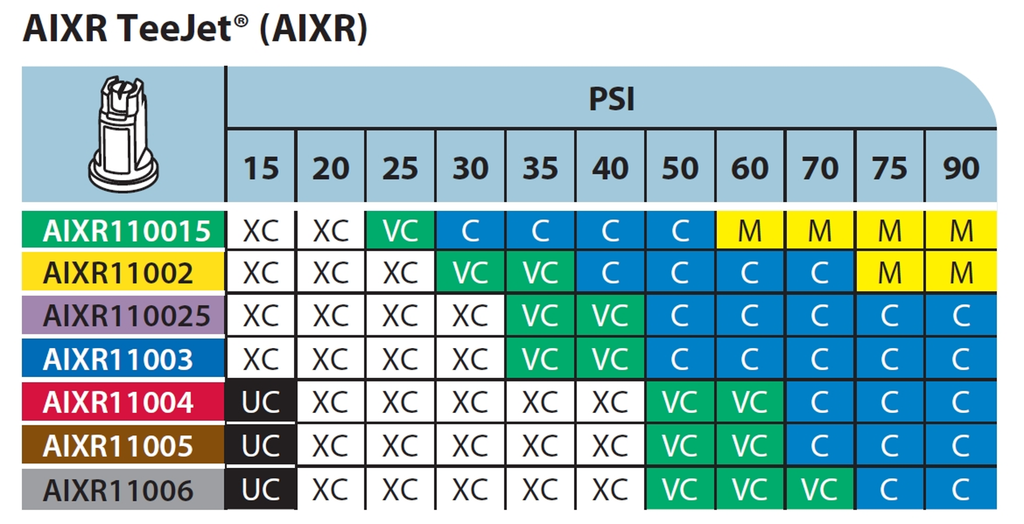
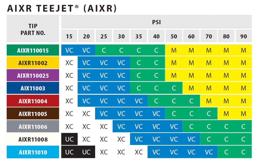
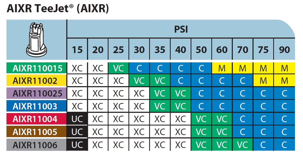
    For example, compare Figure 2, the TeeJet AIXR nozzle spray quality chart, developed using ASABE S572.2 and published in 2015, to Figure 3, the same nozzle whose spray quality was categorized using ASABE S572.3 and published in 2023.

    Figure 2: Spray quality of TeeJet AIXR tips according to S572.2, published by Spraying Systems in 2015. Reproduced from TeeJet Catalog 51A.

    First, let’s compare the portion of the chart that reports Medium spray qualities in Figure 2 to that in Figure 3. These should be the same given that the same boundary nozzle and pressure was used in both. But under the new testing, the region reporting a Medium spray has significantly expanded towards the lower pressures. The Medium sprays begin at 60 and 75 psi in the old standard, but at 50 psi for the new standard.

    Spray quality of TeeJet AIXR tips according to S572.3, published by Spraying Systems in 2023. Reproduced from TeeJet Catalog 52.

    The region occupied by the Coarse category has shifted towards lower pressures, as expected with the coarser upper (C/VC) boundary nozzle. It would be wider, as was the intent, had the M catergory not encroached.

    The region occupied by VC and XC have grown towards the lower left, more or less as expected. The VC category in particular, now dominates in the lower pressure region, a space previously occupied by the XC category. The small region which the UC category occupied under S572.2 in Figure 7 was replaced entirely by the XC category.

    Looking at it another way, the commonly used AIXR11004 size at pressures between 30 and 90 psi would have produced XC, VC, and C spray qualities in the old catalogue. The same nozzle now apparently produces VC, C, and M sprays at the same pressure range.

    These changes may or may not extend across all nozzles and manufacturers to the same extent as this example illustrates. But they add another level of complexity, and perhaps confusion, to applicators striving to be compliant with label directions. I am hopeful that the sector can quickly move to adopt the changes universally so that the mixed messaging is short lived and mistakes are minimized.  

    In particular, the regulatory bodies that rely on these spray quality classes to communicate drift potential and buffer zones must recognize that their risk assessments will need to reflect these new standards as more nozzle manufacturers begin communicating them.

    Droplet size continues to explain most of what matters in spraying, from deposition uniformity, to coverage and spray drift. Hopefully this series of articles explaining the measurement of spray droplet sizes is useful and sheds some light on how the industry measures and communicates it.

  • What is Spray Quality, Part 3 – The Evolution of Standards

    What is Spray Quality, Part 3 – The Evolution of Standards

    When scientists with laser droplet sizing instruments compared their results with other labs using the same nozzles, the numbers didn’t agree exactly. Laser equipment type and age, optics, operating settings, scanning techniques, and software versions were important. Everybody had their own numbers that they trusted more than their colleagues’ in another lab. In order to communicate droplet sizes to the end user consistently, a way to resolve these differences needed to be found.

    Scientists ushered in a new approach, that of using reference nozzles.

    Rather than argue about whose instrument or measurement method was correct, experts decided to allow each lab to use their equipment but with measurement protocols that met certain standards for scanning accuracy. The way the systems were compared was with a set of agreed-on reference nozzles. These reference nozzles defined the boundaries of spray qualities and were measured by the lab at the same time they tested other nozzles. When a nozzle of interest produced a spray whose parameters fell between two reference nozzles, the spray quality was thus defined. In this way, the peculiar results of a certain measurement approach became irrelevant. All that mattered was where the result lay with respect to the reference nozzles tested by the same lab.

    Credit is due to members of the British Crop Protection Council, who pioneered this result in the UK in the mid 1980s, and on which today’s droplet size classification standards are based. Their initial standard was first proposed in this paper:

    Doble S J, Matthews G A, Rutherford 1, Southcombe E S E (1985). A System for Classifying Hydraulic and Other Atomizers Into Categories of Spray Quality. Proceedings British Crop Protection Conference – Weeds, 3, 1125-1133.

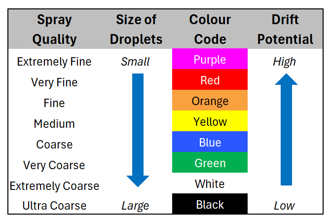
    Thus the term “Spray Quality” was born, and after various incremental revisions, sprays were named Extremely Fine, Very Fine, Medium, Coarse, Very Coarse, Extremely Coarse, and Ultra Coarse and given a colour code for easy identification.

    The American Society of Agricultural and Biological Engineers (ASABE) published the first Spray Quality Standard, S572, in 1999. It specified reference nozzles that formed boundaries from VF/F to VC/XC. It was updated to S572.2 in 2014 with the addition of the Ultra-Coarse category.

    Figure 1: Symbols and colours used to designate spray qualities according to ASABE S572.1 and S572.2

    In order to better represent nozzles that produced finer and coarser sprays, boundary nozzles for XF/VF and XC/UC were introduced with ASABE S572.1 in 2004. ASABE S572.2 corrected an error in the flow rate of the XC/UC in 2014.

    In 2020, ASABE S572.3 was introduced, following on the heels of ISO 25358 that changed the operating conditions for the C/VC, CV/XC, and XC/UC boundary nozzles.  S572.3 and ISO 25358 share the same boundary nozzles, allowing for similar implementation of the spray qualities across borders.

    Table 1: ASABE S572 spray quality categories and their respective boundary nozzles and operating parameters.

    The newest standards changed the boundary nozzle conditions for C/VC, VC/XC, and XC/UC as shown in Table 1. This was done in order to create more equally sized spray quality categories for the coarsest sprays.

    How the Standard is Implemented

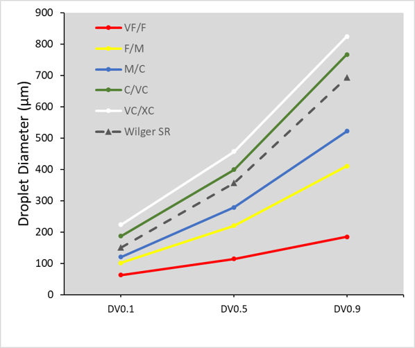
    A laboratory that measures spray qualities would start by running the ASABE reference nozzles on their instrument. They would then calculate the three parameters we described in Part 2 (DV0.1, DV0.5, and DV0.9) and plot them as shown in Figure 2. Next, the lab would atomize various nozzles, pressures, adjuvants, etc. of interest to see where their parameters fall with regard to the reference nozzles and make a spray quality designation. In the example we’ve been showing, the Wilger SR nozzle is in the “Coarse” category using this approach.

    Figure 2: ASABE S572.2  reference nozzles showing spray quality boundaries. Note that the example Wilger SR 11005 tip falls between the Medium/Coarse and the Coarse/Very Coarse border nozzles, making the spray quality “Coarse”.

    Nozzle manufacturers have a responsibility to publish the spray qualities of their nozzles, and they do so on their web sites or catalogues. This makes it much easier for applicators to select the right nozzle for the job. With spray quality, the nozzle brand becomes less important. In fact, nozzles that produce the same spray quality can be expected to have very similar performance. Various nozzle models still have important distinguishing features, such as pressure range, fan angle, pattern tilt, etc. But a 110 degree air-induced nozzle that produces a “Coarse” spray quality should perform very similarly to a different manufacturer’s 110 degree air-induced nozzle that also produces a “Coarse” spray quality.

    Figure 3: Spray qualities of the TeeJet AIXR nozzles according to standard ASABE S572.2. Note the sensitivity of spray quality to both spray pressure and nozzle size. Source: TeeJet catalog 51A.

    Note that the spray quality categories are quite broad. Within any given spray quality range, we might see a two-fold range of drift potential, for example. It remains important to have a sense of where one is operating withing the spray quality range.

    As these standards change, there are implications for how they can be used. An important change occurred with the latest version of the spray quality standard, and that will be discussed in Part 4.